WIXLIB

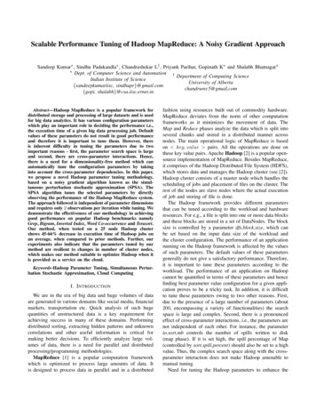
θ3θ1θ0θ θ2Figure 2: Noisy Gradient scheme. Notice that the noise canbe filtered by an appropriate choice of diminishing step sizes.sequence and αn is the step-size. Fig. 2 presents an intuitivepicture of how a noisy gradient algorithm works. Here, thealgorithm starts at θ0 and needs to move to θ which isthe desired optimal solution. The solid lines denote the truegradient step (i.e., αn fn ) and the dash-dotted circles showthe region of uncertainty due to the noise term αn Mn . Thedotted line denotes the fact that the true gradient is disturbedand each iterate is pushed to a different point within theregion of uncertainty. The idea here is to use diminishingstep-sizes to filter the noise and eventually move towardsθ . The simultaneous perturbation stochastic approximation(SPSA) algorithm is a noisy gradient algorithm which worksas illustrated in Fig. 2. It requires only 2 observationsfrom the system per iteration. Thus the SPSA algorithm isextremely useful in cases when the dimensionality is highand the observations are costly. We adapt it to tune theparameters of Hadoop. By adaptively tuning the Hadoopparameters, we intend to optimize the Hadoop job executiontime, which is the performance metric (i.e., f (θ)) in ourexperiments.C. Simultaneous Perturbation Stochastic Approximation(SPSA)We use the following notation:1) θ X Rn denotes the tunable parameter. Here nis the dimension of the parameter space. Also, X isassumed to be a compact and convex subset of Rn .2) Let x Rn be any vector, then x(i) denotes its ithco-ordinate, i.e., x (x(1), . . . , x(n)).3) f (θ) denotes the performance of the system for parameter θ. Let f be a smooth and differentiable functionof θ. f f, . . . , θ(n)) is the gradient of the4) f (θ) ( θ(1) ffunction, and θ(i) is the partial derivative of f withrespect to θ(i).5) ei Rn is the standard n-dimensional unit vector with1 in the ith co-ordinate and 0 elsewhere.Formally the gradient is given by ff (θ hei ) f (θ) lim. θ(i) h 0h(2)In (2), the ith partial derivative is obtained by perturbing theith co-ordinate of the parameter alone and keeping rest of theco-ordinates the same. Thus, we require n 1 operations tocompute the gradient once using perturbations. This can bea shortcoming in cases when it is computationally expensiveto obtain measurements of f and the number of parametersis large.The idea behind the SPSA algorithm is to perturb not justone co-ordinate at a time but all the co-ordinates togethersimultaneously in a random fashion. However, one has tocarefully choose these random perturbations so as to be ableto compute the gradient. Formally, a random perturbation Rn should satisfy the following assumption.Assumption 1: For any i 6 j, i 1, . . . , n, j 1, . . . , n, the random variables (i) and (j) are zeromean,independent, and the random variable Zij given by (i)is such that E[Zij ] 0 and it has finite secondZij (j)moment.An example of such a random perturbation is the following:Let Rn be such that, each of its co-ordinates (i)is an independent Bernoulli random variable taking values 1 or 1 with equal probability, i.e., P r{ (i) 1} P r{ (i) 1} 21 for all i 1, . . . , n. This randomvariable satisfies Assumption 1.D. Noisy Gradient Recovery from Random Perturbationsˆ θ denote the gradient estimate, and let RnLet fbe any perturbation vector satisfying Assumption 1. Thenfor any small positive constant δ 0, the one-sided SPSAalgorithm [9] obtains an estimate of the gradient accordingto equation (3) given below.ˆ θ (i) f (θ δ ) f (θ) . fδ (i)(3)ˆ θ (i), which is givenWe now look at the expected value of fby the following:ˆ θ (i) θ] f o(δ).(4)E[ f θ(i)Thecan be easily computed, sinceh above equationi f (j)E θ(j) θ 0.Thisfollows from the property of (i)ˆ θ (i)] fθ (i) as δ 0. in Assumption 1. Thus E[ fNotice that in order to compute the gradient fθ at the pointθ the SPSA algorithm requires only 2 measurements namelyf (θ δ ) and f (θ δ ). An extremely useful consequenceis that the gradient estimate is not affected by the numberof dimensions. The complete SPSA algorithm is shown inAlgorithm 1, where {αn } is the step-size schedule and Γ isa projection operator that keeps the iterates within X.Algorithm 1 uses a noisy gradient estimate (in line 6)and at each iteration takes a step in the negative gradientdirection so as to minimize the cost function. The noisygradient update can be re-written as ˆ n θn ] fˆ n E[ fˆ n θn ])θn 1 Γ θn αn E[ f(5) Γ θn αn fn Mn 1 n )

Algorithm 1 Simultaneous Perturbation Stochastic Approximation1: Let initial parameter setting be θ0 X Rn2: for n 1, 2 . . . , N do3:Observe the performance of system f (θn ).4:Generate a random perturbation vector n Rn .5:Observe the performance of system f (θn δ n ).ˆ n (i)6:Compute the gradient estimate f f (θn δ n ) f (θn δ n ).2 δ n (i)7:Update the parameter in the negative gradient direcn ) f (θn )tion θn 1 (i) Γ θn (i) αn f (θn δ .δ n (i)8: end for9: return θN 1ˆ n E[ fˆ n θn ] is an associated marwhere Mn 1 ftingale difference sequence under the sequence of σ-fieldsFn σ(θm , m n, m , m n), n 1 and n is a smallbias due to the o(δ) term in (4). The iterative update in (5)is known as a stochastic approximation [10] recursion. Asper the theory of stochastic approximation, in order to filterout the noise, the step-size schedule {αn } needs to satisfythe conditions below. Xn 0αn , Xαn2 .(6)n 0The first of the conditions in (6) ensures that the algorithmdoes not converge to a non-optimal parameter configurationprematurely, while the second ensures that the noise asymptotically vanishes. If the above conditions are satisfied, theiterates of the algorithm converge to local minima (see [10]).However, in practice local minima corresponding to smallvalleys are avoided due either to the noise inherent in theupdate or one can periodically inject some noise so as to letthe algorithm explore further. Also, though the result statedin [10] is only asymptotic in nature, in most practical casesconvergence is observed in a finite number of steps.E. Adapting SPSA Algorithm to tune Hadoop ParametersThe performance of an application running on Hadoop canbe measured by different metrics - namely amount of memory used, number of jobs spawned, execution time etc. Outof these, measuring the execution time of a job is the mostpractical, as it gives an idea about the job dynamics. Ourmethod involves adapting SPSA algorithm to improve theexecution time of jobs running on Hadoop/Hive. Thus, withrespect to Section II B, the function f (θ) hereon denotes theexecution time of a workload for a given parameter vector θ.We believe that this multi-variate function representing theexecution time of a workload is multimodal and has multiplelocal minima (we do not assume any form of the function like convexity, or non-linear). Thus, finding a local minimais as good as finding a global minimizer. All minima of thefunction lead to a similar performance with respect to theexecution time.The SPSA algorithm needs each of the parameter components to be real-valued i.e., θ X Rn . However,most of the Hadoop parameters that are of interest arenot Rn -valued. Thus, on the one hand we need a set ofRn -valued parameters that the SPSA algorithm can tuneand a mapping that takes these Rn -valued parameters tothe Hadoop parameters. In order to make things clear weintroduce the following notation:1) The Hadoop parameters are denoted by θH and theRn -valued parameters tuned by SPSA are denoted byθA 1 .2) Si denotes the set of values that the ith Hadoopminmaxdparameter can assume. θH(i), θH(i) and θH(i)denote the minimum, maximum and default values thatthe ith Hadoop parameter can assume.3) θA X Rn and θH S1 . . . Sn .4) θH µ(θA ), where µ is the function that maps θA X Rn to θH S1 . . . Sn .In this paper, we choose X [0, 1]n , and µ : θ Rnsuch that µ(θA )(i) y, wheremaxminminy (θH(i) θH(i))θA (i) θH(i). For an integer valued parameter, we let µ(θA )(i) byc.We chose δ n Rn to be independent random variables,1} P r{δ n (i) such that P r{δ n (i) θmax (i) θminHH (i)11 θmax (i) θmin (i) } 2 . This perturbation sequence ensuresHHthat the Hadoop parameters assuming only integer valueschange by a magnitude of at least 1 in every perturbation.Otherwise, using a perturbation whose magnitude is less1might not cause any change to thethan θmax (i) θminHH (i)corresponding Hadoop parameter resulting in an incorrectgradient estimate.The conditions for the step-size schedule {αn } are asymptotic in nature and are required to hold for convergence tolocal minima. However, in practice, a constant step sizecan be used since one reaches closer to the desired valuein a finite number of iterations. We know apriori that theparameters tuned by the SPSA algorithm belong to theinterval [0, 1] and it is enough to have step-sizes of the1order of mini ( θmax (i) θ) (since any finer step-sizeminHH (i)used to update the SPSA parameter θA (i) will not causea change in the corresponding Hadoop parameter θH (i)). Inour experiments, we chose αn 0.01, n 0 and observedconvergence in about 20 iterations.III. E XPERIMENTAL E VALUATIONIn this paper, we have used use Hadoop versions 1.0.3,2.7.3 and Hive version 2.1.1 for our experiments. First,we justify the selection of parameters to be tuned in our1 Here subscripts A and H are abbreviations of the keywords Algorithmand Hadoop respectively

experiments. Then, we give details about the implementationfollowed by discussion of results.A. Parameter SelectionHadoop consists of myriad of tunable parameters, however most of them are concerned with Hadoop setup andbookkeeping activities and does not affect the performanceof workloads. Based on the data flow analysis of HadoopMapReduce (see [2]) we identify 11 parameters whichare found to critically affect the operation of HDFS andthe Map/Reduce operations (listed in Table I). We tuneparameters which are directly Hadoop dependent, for e.g.,number of reducers, I/O utilization parameter etc. and avoidtuning parameters, which are not directly related to Hadoopsuch as mapred.child.java.opts which are best left for clusteror OS level optimization.B. Cluster Setup and BenchmarksOur Hadoop cluster consists of 25 nodes. Each node hasa 8 core Intel Xeon E3, 2.50 GHz processor, 3.5 TB HDD,16 GB memory and Gigabit connectivity.In order to evaluate the performance of our method, weuse representative benchmark applications. Terasort takesas input a text data file (generated using teragen) andsorts it. Grep searches for a particular pattern in a giveninput file. Bigram counts all unique sets of two consecutivewords in a set of documents, while Inverted Index generatesword to document indexing from a list of documents. WordCo-occurrence is a popular Natural Language Processingprogram which computes the word co-occurrence matrix ofa large text collection.C. Hive WorkloadMapReduce, although capable of processing hugeamounts of data, is often used with a wrapper around it toease its usage. Hive [11] is one such wrapper which providesan environment where MapReduce jobs can be specifiedusing SQL. Its performance can be tested on clusters usingthe TPCDS benchmark. This benchmark generates data(scale factor) as per requirement and executes a suite of SQLqueries on the generated data. The SQL queries focus on different aspects of performance. In our experiments, we haveselected 4 queries, which are first optimized using SPSA(see Fig. 3). Following this, we compare the performance ofTPCDS using the parameters tuned by SPSA algorithm andvalues suggested in the TPCDS manual (see Fig. 4d).D. Learning/Optimization PhaseSPSA runs a Hadoop job with a different configuration ineach iteration. We refer to these iterations as the optimizationor the learning phase. The algorithm eventually convergesto an optimal value of the configuration parameters. The jobexecution time corresponding to the converged parametervector is optimal for the corresponding application. Duringour evaluations we have seen that SPSA algorithm convergeswithin 10 - 15 iterations and within each iteration it makestwo observations, i.e. it executes Hadoop job twice, takingthe total count of Hadoop runs during the optimization phaseto 20 - 30. It is of utmost importance that the optimizationphase is fast, otherwise it can overshadow the benefits whichit provides.Partial Data: In order to ensure a fast optimizationphase, we execute the Hadoop jobs (during this phase) on apartial workload. Deciding the size of this partial workload(denoted Np ) is crucial as the run time on a small work loadwill be eclipsed by the job setup and cleanup time. We takecue from Hadoop processing system to determine the size ofthe partial workload. Hadoop splits the input data based onthe block size (denoted bS ) of HDFS and spawns a map foreach of the splits. The number of map tasks that can run inparallel at a given time is upper bounded by the total mapslots (denoted m) available in the cluster. Using this fact,we set the size of the partial data set as:Np 2 bS mUsing workload of this size, Hadoop will use two wavesof the maps jobs to finish the map operation. That willallow SPSA algorithm to capture the statistics of a singlewave and the correlations between two successive waves.Our expectation (and as borne by our results) is that the valueof configuration parameters which optimize these two wavesof map jobs also optimize all the subsequent waves as thoseare repetitions of similar map jobs. In the cases of Bigramand Inverted Index benchmark, we observed that even withsmall amount of data, the job take a long time finish, as theyare reduce-intensive benchmarks. So, while training thesebenchmarks, we have used small sized input data files, whichresults in absence of two waves of map tasks. However, sincein these applications, reduce operations take precedence, theabsence of two waves of map tasks did not create much ofa hurdle.E. Experimental SetupWe optimize Terasort using a partial data set of size30GB, Grep on 22GB, Word Co-occurrence and InvertedIndex on 1GB and Bigram count on 200M B of data set. ForWord-Cooccurrence, Grep and Bigram benchmarks we usethe Wikipedia dataset of 50GB [5]. We use the defaultconfiguration of the parameters as the initial point for theoptimization during the learning/optimization phase.SPSA algorithm terminates when either the change ingradient estimate is negligible or the maximum number ofiterations have been reached. An important point to note isthat Hadoop parameters can take values only in a fixed range.We handle this by projecting the tuned parameter values intothe range set (component-wise).

F. Discussion of ResultsWe compare our method with Starfish [4] and Profilingand Performance Analysis-based System (PPABS) [6] frameworks. Starfish is designed for Hadoop v1 only, whereasPPABS works with the recent versions also. To run Starfish,we use the executable hosted by the authors of [4] to profilethe jobs run on partial workloads. Then execution time ofnew jobs is obtained by running the jobs using parametersprovided by Starfish. For testing PPABS, we collect and usethe datasets as described in [6].1) Performance Evaluation: Our method initializes theparameters to the default values. The execution time corresponding to this initial parameter configuration is given byfirst data point in all plots of Fig. 3. The initial variationin the execution times of the benchmarks is due to thenoisy nature of the gradient estimate. These eventually diedown after a few iterations. Since the execution times of theapplications are stochastic in nature, we run 10 Monte Carlosimulations with the optimal parameters tuned by SPSA.This gives us the average execution time as well as thestandard deviation for each benchmark.As can be observed from Fig. 4, SPSA reduces theexecution time of Terasort benchmark by 60% 63%when compared to default settings and by 40% 60%when compared to Starfish optimizer. For Inverted Indexbenchmark the reduction is about 80% when compared todefault settings and about 40% when compared to Starfish.In the case of Word Co-occurrence, the observed reductionis 70% when compared to default settings and 50% whencompared to Starfish.SPSA, while finding the optimal configuration, factorsin the co-relation among the parameters (Table I). Forexample, in Terasort, a small value (0.14 or 14%) ofio.sort.spill.percent will generate a lot of spilled files ofsmall size. Because of this, the value of io.sort.factor hasbeen increased to 475 from the default value of 10. This willensure that a large number of spilled files (475) are combined to generate the partitioned and sorted file. Similarly,shuffle.input.buffer.percent and inmem.merge.threshold (0.14and 9513 respectively) act as a threshold beyond which inmemory merge of files (output by map) is triggered. Becauseof low value of io.sort.spill.percent the size of the spilledfiles will be small, and it would take a large number of files(9513) to fill the 14% of reduce memory.Default value of number of reducers (i.e., 1) generallydoes not work in practical situations. However, increasing itto a very high number also creates an issue as it results inmore network and disk overhead. SPSA optimizes this basedon the map output size. Grep benchmark, produces verylittle map output, and even smaller sized data to be shuffled.Hence io.sort.mb value is reduced to 50 from default 100(see Table I) and number of reducers is set to 1. Further,value of inmem.merge.threshold has been reduced to 681from 1000 as there is not much data to work on.The difference in the values of the tuned parameter inHadoop 1 and Hadoop 2 for the same benchmark arisesbecause of inherent differences in their architecture and howjobs are executed.2) Dynamically Changing Cluster Configuration: Thetuning of parameters by SPSA is independent of the numberof nodes in the cluster. This is substantiated by the resultsshown in Fig. 4c, which shows the execution times ofbenchmark applications when the number of nodes in thecluster was reduced to half. The parameter values providedby SPSA are same as the optimal values provided by it, forthe original cluster configuration (as described in SectionIII-B). The execution times (in seconds) for the benchmarkapplications, based on multiple Monte Carlo simulations are:Terasort: 456 13.12, Bigram: 630 17, Inverted Index:251 4.2 and Word Co-occurrence: 2786.4 16.9.The tuning of parameters by SPSA depends on the configuration of the nodes (which is not changed when nodesare added or removed), as some Hadoop parameters likeio.sort.mb are influenced by memory available in each node.The lack of dependency on number of nodes in the clustercomes from the fact that SPSA optimizes the performance ofa single map or reduce wave. This results in optimization ofall subsequent waves. Addition or removal of nodes meansthere will be less or more number of map-reduce waves.3) Comparison against Random Configuration: As asanity check, we compare the performance of SPSA againsta random setting of the configuration parameters. Whencompared with default setting, where the number of reduceris 1, one can get a better performance by just increasing thisnumber. However, that is not optimal and can be improvedfurther by using a more mathematical proven techniques likeSPSA. The results (average of 5 executions) are shown infigure 4c. One issue with random setting is that sometimeit will lead

these key value pairs. Apache Hadoop [2] is a popular open-source implementation of MapReduce. Besides MapReduce, it comprises of the Hadoop Distributed File System (HDFS), which stores data and manages the Hadoop cluster (see [2]). Hadoop cluster consists of a master node which handles the scheduling of jobs and placement of files on the .