WIXLIB

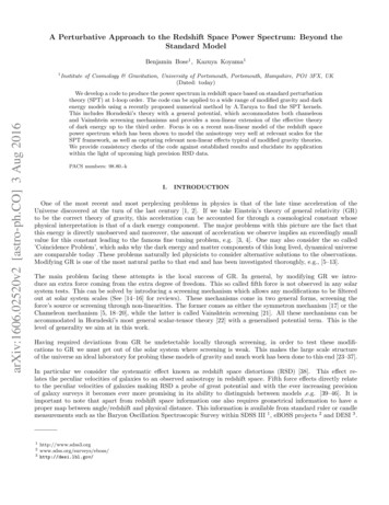
A Perturbative Approach to the Redshift Space Power Spectrum: Beyond theStandard ModelBenjamin Bose1 , Kazuya Koyama1arXiv:1606.02520v2 [astro-ph.CO] 3 Aug 20161Institute of Cosmology & Gravitation, University of Portsmouth, Portsmouth, Hampshire, PO1 3FX, UK(Dated: today)We develop a code to produce the power spectrum in redshift space based on standard perturbationtheory (SPT) at 1-loop order. The code can be applied to a wide range of modified gravity and darkenergy models using a recently proposed numerical method by A.Taruya to find the SPT kernels.This includes Horndeski’s theory with a general potential, which accommodates both chameleonand Vainshtein screening mechanisms and provides a non-linear extension of the effective theoryof dark energy up to the third order. Focus is on a recent non-linear model of the redshift spacepower spectrum which has been shown to model the anisotropy very well at relevant scales for theSPT framework, as well as capturing relevant non-linear effects typical of modified gravity theories.We provide consistency checks of the code against established results and elucidate its applicationwithin the light of upcoming high precision RSD data.PACS numbers: 98.80.-kI.INTRODUCTIONOne of the most recent and most perplexing problems in physics is that of the late time acceleration of theUniverse discovered at the turn of the last century [1, 2]. If we take Einstein’s theory of general relativity (GR)to be the correct theory of gravity, this acceleration can be accounted for through a cosmological constant whosephysical interpretation is that of a dark energy component. The major problems with this picture are the fact thatthis energy is directly unobserved and moreover, the amount of acceleration we observe implies an exceedingly smallvalue for this constant leading to the famous fine tuning problem, e.g. [3, 4]. One may also consider the so called’Coincidence Problem’, which asks why the dark energy and matter components of this long lived, dynamical universeare comparable today .These problems naturally led physicists to consider alternative solutions to the observations.Modifying GR is one of the most natural paths to that end and has been investigated thoroughly, e.g., [5–13].The main problem facing these attempts is the local success of GR. In general, by modifying GR we introduce an extra force coming from the extra degree of freedom. This so called fifth force is not observed in any solarsystem tests. This can be solved by introducing a screening mechanism which allows any modifications to be filteredout at solar system scales (See [14–16] for reviews). These mechanisms come in two general forms, screening theforce’s source or screening through non-linearities. The former comes as either the symmetron mechanism [17] or theChameleon mechanism [5, 18–20], while the latter is called Vainshtein screening [21]. All these mechanisms can beaccommodated in Horndeski’s most general scalar-tensor theory [22] with a generalised potential term. This is thelevel of generality we aim at in this work.Having required deviations from GR be undetectable locally through screening, in order to test these modifications to GR we must get out of the solar system where screening is weak. This makes the large scale structureof the universe an ideal laboratory for probing these models of gravity and much work has been done to this end [23–37].In particular we consider the systematic effect known as redshift space distortions (RSD) [38]. This effect relates the peculiar velocities of galaxies to an observed anisotropy in redshift space. Fifth force effects directly relateto the peculiar velocities of galaxies making RSD a probe of great potential and with the ever increasing precisionof galaxy surveys it becomes ever more promising in its ability to distinguish between models ,e.g. [39–46]. It isimportant to note that apart from redshift space information one also requires geometrical information to have aproper map between angle/redshift and physical distance. This information is available from standard ruler or candlemeasurements such as the Baryon Oscillation Spectroscopic Survey within SDSS III 1 , eBOSS projects 2 and DESI 3 /http://desi.lbl.gov/

2Consequently, with the heightened precision of recent and upcoming surveys, theory is required to keep up interms of its predictive power. Even though made at linear to quasi linear scales, non-linearities of the gravitationalinteraction play an important role in the RSD observations and a lot of work has been done on modelling RSDbeyond the linear Kaiser model, e.g.[47–52]. This non-linear dependence makes it crucial to properly model RSDwhen changing the structure of gravity in order to get the correct and distinguishing predictions. In this work wegive attention to an improved RSD model developed in Ref.[52] which we call the TNS model after its authors. Themodel uses standard perturbation theory (SPT) to construct the non-linear redshift space power spectrum and hasbeen shown to perform very well when compared to N-body simulations [53–55].It is worth discussing the overlap and distinction between modified gravity effects and the flexibility of standard GR templates, i.e. nuisance parameters such as galaxy or halo bias, when we consider the redshift space powerspectrum. Whether the standard GR treatment gives biased results for the constraints on modified gravity modelparameters or not depends on the method used in modelling RSD and also the precision of the measurements.Clearly, if the errors in the measurements are larger than the bias introduced by the inaccurate modelling of RSD,there is no need to improve the RSD modelling. However this needs to be tested before the method is applied toreal data. For the TNS model, which has been used to measure f σ8 using the power spectrum measurements ofBOSS survey [56], this has been done only for f (R) gravity. In this model, it was shown that the standard GRtemplate gives a biased estimation of the model parameter assuming an ideal survey with volume 10Gpc3 h 3 atz 1 [54]. Thus, it is important to test whether this kind of bias exists for other MG models. In Ref.[57] theyfind that with their analysis of the redshift space power spectrum for a Vainshtein screened model, no model bias isfound. The expectation is that this absence of model bias is true for scale independent models of gravity (unlike thescale dependent f (R) case). In a future work we will test for consistency with this result. For this, clearly we needto develop the TNS model including the modified gravity effect consistently.Recently a method to find the SPT kernels numerically was developed in Ref.[58]. In the work the authorsapply this method to calculate the real space power spectrum for GR and the f (R) model of gravity. Here, wepresent a new code which follows their method for computing the perturbative kernels up to 3rd order and thenextends their work in applying the kernels to calculate the TNS redshift space power spectrum. The code also usesthe general applicability of the numerical method to accommodate a large class of gravity and dark energy models. Inparticular, we describe and show results for our code’s application to a Vainshtein screened and chameleon screenedmodel, namely the DGP model of gravity [7] and the Hu-Sawicki form of f (R) gravity [5].This paper is organised as follows: In Sec.II we review the relevant theory. We start by deriving the generalised evolution equations for the velocity and density perturbations, highlighting where the modifications to GRarise, parametrizing these modifications in terms of 1st, 2nd and 3rd order effects. We also present expressions forthe 1-loop auto and cross real space power spectra in terms of the 1st , 2nd and 3rd order perturbation kernels. AChameleon and Vainshtein screened model are given as explicit examples under our parametrisation. We finish thesection with a review of the TNS model of RSD, giving the analytical expressions in terms of our generalised SPTkernels. In Sec.III we detail our code and provide some results. First we compare the code’s results for the 1-loopreal space power spectrum and TNS monopole with well established analytical results in SPT for both GR and aVainshtein screened model of gravity. This is done as a consistency check. Next we compare the code’s results withN-body results for a Chameleon screened model of gravity in an attempt to reproduce some of the results of Ref.[59].Finally, we summarise our results and highlight future work in Sec.V.II.A.THEORYEvolution equations for the perturbationsWe consider perturbations around the Friedman-Robertson-Walker (FRW) universe described in the Newtoniangauge.ds2 (1 2Φ)dt2 a2 (1 2Ψ)δij dxi dxj .(2.1)We will work on the evolution of matter fluctuations inside the Hubble horizon. Then we can use the quasi-staticapproximation and neglect the time derivatives of the perturbed quantities compared with the spatial derivatives. Asmentioned in the introduction, the large distance modification of gravity which is necessary to explain the late-timeacceleration generally modifies gravity even on sub-horizon scales due to the introduction of a new scalar degree

3of freedom. In this paper, we use the Jordan frame where matter is minimally coupled to gravity. The evolutionequations for matter perturbations are obtained from the conservation of the energy momentum tensor. This givesthe continuity and Euler equations.1 δ · [(1 δ)v] 0, ta v11 Hv (v · )v Φ. taa(2.2)(2.3)Assuming the irrotationality of fluid quantities, the velocity field v is expressed in terms of velocity divergenceθ · v/(a H). Then the Fourier transform of the fluid eq.(2.2) and eq.(2.3) becomeZ 3 δ(k)d k1 d3 k2δD (k k1 k2 )α(k1 , k2 ) θ(k1 )δ(k2 ),(2.4)a θ(k) a(2π)3 2Z 31 θ(k)aH 0kd k1 d3 k2Φ(k) δD (k k1 k2 )β(k1 , k2 ) θ(k1 )θ(k2 ), (2.5)a 2 θ(k) aHaH2(2π)3the prime denoting a scale factor derivative and the kernels in the Fourier integrals, α and β, are given byα(k1 , k2 ) 1 k1 · k2, k1 22β(k1 , k2 ) (k1 · k2 ) k1 k2 . k1 2 k2 2(2.6)The information on modifications of gravity is encoded in the relation between the Newtonian potential Φ and δ. Inorder to calculate the non-linear power spectrum at 1-loop order using SPT, we need to expand δ up to the thirdorder using SPT (See Ref.[60] for a review). We assume the Newtonian potential is related to δ non-linearly and weexpand this relation up to the third order [61] 2k3Ωm (a) Φ µ(k, a) δ(k) S(k),(2.7)aH2where Ωm (a) 8πGρm /3H 2 . The function S(k) is the non-linear source term up to the third order given byZ 3d k1 d3 k2S(k) δD (k k12 )γ2 (k, k1 , k2 ; a)δ(k1 ) δ(k2 )(2π)3Z 3d k1 d3 k2 d3 k3 δD (k k123 )γ3 (k, k1 , k2 , k3 ; a)δ(k1 ) δ(k2 ) δ(k3 )(2π)6(2.8)where γ2 (k, k1 , k2 ; a) and γ3 (k, k1 , k2 , k3 ; a) are symmetric under the exchange of ki .We solve eq.(2.4) and eq.(2.5) perturbatively. The n-th order solutions are given byZδn (k, a) d3 k1 .d3 kn δD (k k1.n )Fn (k1 , ., kn , a)δ0 (k1 ).δ0 (kn )Zθn (k, a) d3 k1 .d3 kn δD (k k1.n )Gn (k1 , ., kn , a)δ0 (k1 ).δ0 (k2 )(2.9)(2.10)where k1.n k1 . kn . In the following we will omit the scale factor dependence of the kernels to simplify theexpressions.By insterting eq.(2.9) and eq.(2.10) into the continuity and Euler equations we get a generalised form of thesystem for the nth order kernel (See Ref. [58] for more details) L̂(k)Fn (k1 , · · ·, kn )Gn (k1 , · · ·, kn ) n 1X j 1 α(k1···j , kj 1···n )Gj (k1 , · · ·, kj )Fn j (kj 1 , · · ·, kn ) 21 β(k1···j , kj 1···n )Gj (k1 · · · kj )Gn j (kj 1 , · · ·, kn ) Nn (k, k1 , · · ·, kn ) (2.11)whereL̂(k) da da 13Ωmdµ(k,a)a 2 2da!aH 0H (2.12)