WIXLIB

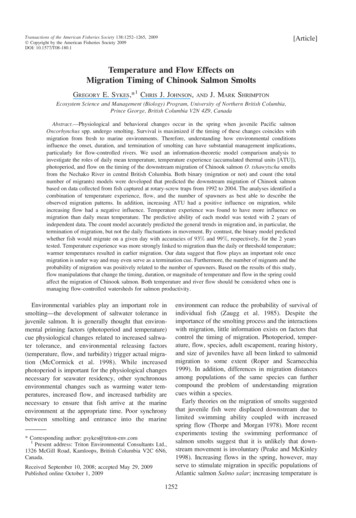
ENVIRONMENTAL CONTROL OF SMOLT MIGRATIONthe dataset. We used a Vuong test to compare theoutput of a NBRM to that of a ZINB and determinewhether a zero-inflated model was necessary (Vuong1989). All statistics were completed using Stata version9.2 (Statacorp, College Station, Texas).Model parameters.—We developed candidate models from a small set of predictor variables recognized asimportant for explaining the timing of migration ofjuvenile Chinook salmon: temperature (8C), accumulated thermal units (ATU, sum of daily meantemperatures [8C]), flow (m3/s), and photoperiod (hoursof daylight per day). In addition to combinations ofthese variables, all binary and count models included aterm representing the number of spawners, a factor thatcan influence year-to-year variation in migrationnumbers and also the probability of migration. Thebrood year for migrating Chinook salmon in theNechako River is 2 years before the date of migration.Additionally, a quadratic equation was used to describevariables that have a nonlinear distribution during themigration period such as temperature and ATU. Allparameters with the exception of that for spawnerswere tested to see whether use of a quadratic equationwas appropriate; however, only temperature2 andATU2 resulted in a lower small-sample-bias-correctedAkaike’s information criterion (AICc) score than in thesame model with only the linear parameter.Both mean daily water temperature data and flowdata were collected from the Water Survey of Canada(WSC) station located upstream from the trap site nearCheslatta Falls (Station 08JA017). Although thisstation is located approximately 70 rkm upstream fromthe trap site, it is the most reliable and continuousdataset available for the upper Nechako River andprovided a record of river temperatures before trapinstallation, which was important for calculating ATUs.The gauge data are considered representative ofconditions at the trap site due to the lack of largetributaries between the two sites and the fact that thegauge is upstream from the traps. Comparison of datacollected at the trap site and at the WSC station fordays when both were available did not show asignificant difference in mean daily temperature (P ¼0.1) or flow (P ¼ 0.08). Accumulated thermal unitswere calculated beginning on March 9, the date onaverage (1987–2004) where mean daily water temperature first reached 18C for the year. Photoperiod datawere calculated for the latitude and longitude of thenearest residential community to the trapping site (FortFraser, British Columbia; 54804 0 N, 124833 0 W). Thenumber of spawners was determined by aerial surveyscompleted by Fisheries and Oceans Canada during thespawning period each year.1255Models.—We developed 11 models (Table 1) torepresent biologically plausible hypotheses to explainjuvenile Chinook salmon migration. During the modeldevelopment stage, the collinearity of the variables wasassessed because in situations where two or morevariables have a strong collinear relationship, aninfinite number of regression coefficients can begenerated that will work equally well in the modelproduced (Menard 2001). We used a linear regressionto calculate tolerance statistics for each of theparameters in the model. A tolerance statistic isequivalent to 1 R2 and values less than 0.1 suggeststrong collinearity (Menard 2001). An initial assessment of collinearity identified a linear relationshipbetween ATU2 and temperature2 (tolerance value of0.20 and 0.12, respectively). As a result, no modelswere tested that included both of those variables. Thetolerance scores for the remaining combinations ofvariables exceeded 0.3 and, therefore, collinearity wasnot considered a problem.Model selection.—Applying the ITMC technique,we used AIC to identify the most parsimonious model.The AICc form, which is corrected for small-samplebias, was used in place of the standard AIC value asAICc has been shown to converge to the standard AICvalue as the sample size increases (Burnham andAnderson 2004). The formula for calculating AICc is asfollows:AICc ¼ 2LL þ 2K þ 2K ðK þ 1Þ ðn K 1Þ;where LL is the log likelihood, K is the number ofparameters, and n is the sample size. The term Direpresented the difference in AICc between the mostparsimonious model and all subsequent models. If Di isless than 2, models are too similar to be ranked and themodel with the fewest parameters can be selected(Anderson et al. 2000). Also, we report the AIC weight(AICw) for each model. This value represents theprobability that the corresponding model is the bestmodel of the set of tested models. For each parameter,we summed the AICw values from all models thatcontained that parameter; this sum measures therelative importance of each parameter across the modelset. For the best binary and count models, a bcoefficient was generated for each parameter, the signof which corresponded to the direction of the effect.We used the Z-statistic to assess the statisticalsignificance of the individual parameters. Significancewas determined as P , 0.05.Predictive ability.—As recommended by Guthery etal. (2005), we used migration data withheld frommodel construction (years ¼ 1992 and 2004) to conductan independent validation of the most parsimoniousmodels. For the binary analysis, the following binary

1256SYKES ET AL.TABLE 1.—Model selection statistics for the candidate binary and ZINB count models to predict the downstream migration ofjuvenile Nechako River Chinook salmon. For models with a quadratic term, the linear component of the parameter was alsoincluded; ATU ¼ accumulated thermal units.RankAICcDAICcAICwBinaryATU2 þ flow þ photoperiod þ spawnersATU2 þ flow þ spawnersATU2 þ spawnersATU2 þ photoperiod þ spawnersTemperature2 þ flow þ spawnersTemperature2 þ flow þ photoperiod þ spawnersTemperature2 þ photoperiod þ spawnersTemperature2 þ spawnersFlow þ photoperiod þ spawnersPhotoperiod þ spawnersFlow þ 0000.000ZINBATU2 þ flow þ spawners2ATU þ flow þ photoperiod þ spawnersTemperature2 þ flow þ spawnersTemperature2 þ flow þ photoperiod þ spawnersATU2 þ photoperiod þ spawnersATU2 þ spawnersTemperature2 þ photoperiod þ spawnersFlow þ spawnersTemperature2 þ spawnersFlow þ photoperiod þ spawnersPhotoperiod þ 000.0000.0000.0000.000Modellogit model was used to generate the predictedprobability of Chinook salmon migration:Y¼expðb0 þ b1 x1 þ b2 x2 þ þ bi xi Þ;1 þ expðb0 þ b1 x1 þ b2 x2 þ þ bi xi Þwhere b0 is the intercept term, bi is the coefficient foreach covariate in the model, and xi is the value of thecovariate. Pearson’s standardized residuals were usedto assess the difference between the observed andpredicted values. Standardized residuals have a normaldistribution and therefore should have a mean of 0 anda standard deviation (SD) of 1. In addition, 95% of theresiduals should fall between 2 and 2 with larger andsmaller values identifying cases where the modelworks poorly or that exert more than their share ofinfluence on the model parameters (Menard 2001).We used the receiver operating characteristic (ROC)curve and withheld data to evaluate the proportion ofcorrectly and incorrectly classified migration events(Pearce and Ferrier 2000). The general guidelines forinterpreting the area under the ROC curve with respectto predictive ability are: poor (0.5–0.7), reasonable(0.7–0.9), and very good (0.9–1.0) (Swets 1988). Forthe count analysis, we used the Stata programprcounts.ado (Long and Freese 2006) to predict thenumber of migrating salmon. Due to nonnormality ofthe data, a nonparametric Wilcoxon rank-sum test wasused to compare observed and predicted counts for1992 and 2004.ResultsThe negative binomial regression model (NBRM)was preferable to the Poisson regression model (PRM)because of overdispersed count data (G2 ¼ 3180.01, P, 0.001). In addition, when the NBRM and the ZINBwere compared, the large number of zero countsresulted in a better fit for the ZINB (Vuong test ¼ 0.98,P ¼ 0.16). Although not significant, the result wasconfirmed by lower AICc scores and better predictiveability of the ZINB compared with the same modelcalculated using the NBRM.Based on AICc scores, a combination of ATU2, flow,photoperiod, and spawners best modeled the probability of Chinook salmon migration (binary analysis;Table 1). Models that included spawners as a variableconsistently had lower AICc scores than the comparable model without spawners included. Whether spawners was included or not, however, did not change therank of the models. Consequently, spawners wasincluded in all binary models. The second-rankedbinary model (ATU2 þ flow þ spawners) had an AICcscore only 0.6 points greater than the model rankedfirst and, because of the marginal difference in AICcscores, we determined the best model to be the onewith the fewest variables. For the count analysis, thesame two models were ranked first and second basedon AICc score except that the model ranked first (ATU2þ flow þ spawners) was also the simplest and thereforewas selected (Table 1). The combined AICw of each of

1257ENVIRONMENTAL CONTROL OF SMOLT MIGRATIONTABLE 2.—Regression outputs for binary and count models to predict the downstream migration of juvenile Nechako RiverChinook salmon; ATU ¼ accumulated thermal units.95% confidence limitsVariablebSEATUATU2FlowSpawnersConstant0.0126 2 3 10 5 0.01420.00071.4890.00253.6 3 10 83 1.7 3 10 5 0.01190.00031.39850.0011.8 3 10 60.00143.9 3 10 50.1457ATUConstant0.0178 11.1827ZPLowerUpperBinary model4.97,0.001 7.80,0.001 5.93,0.0014.57,0.0013.56,0.0010.0077 3.51 3 10 5 0.19250.00040.66820.01762 2.10 3 10 5 0.00920.00102.3092Count model8.08,0.001 9.31,0.001 8.60,0.0019.81,0.0019.60,0.0010.0063 2.1 3 10 5 0.01470.00031.11290.0103 1.4 3 10 6 0.00920.00051.68410.0119 14.80560.0241 7.5599Count model (inflate portion)0.00325.59,0.0011.8484 6.05,0.001the variables showed ATU2 and flow had a score of1.0, which was higher than any of the other variableswith the exception of that for spawners, which hadbeen included in all other models.Beyond the models ranked first and second, therankings of the remaining models differ for the twodistributions. In the case of the binary model, thevariable ATU2 was found in each of the top fourmodels, with temperature2 found in the following four(ranked 5–8). In the case of the count model, thevariable flow was included in each of the top fourmodels and similar to the binary models, ATU2 wasfound to result in lower AICc scores than thecorresponding temperature2 model.Model CoefficientsThe coefficients generated for each of the variablesincluded in the most parsimonious binary and countmodels (Table 2) had a statistically significant affect onmigration (P , 0.001). Pearson’s standardized residuals for the binary analysis indicated that no recordsinfluenced the model disproportionately (mean ¼0.002, SD ¼ 0.97; 96% of the values being between 2 and þ2). For both the binary and count models,flow and the squared component of the ATU quadraticwere found to have a negative influence on migration,while the linear component of the ATU quadratic, andspawners had a positive influence.We also considered the combined effects of flow andATU, as changes in these variables do not generallyoccur independently. Results of the modeling analysissuggest that both high flow and warmer temperaturesare correlated with a decline in migration. Therefore,years with high ATU and high flow would be expectedto have a shorter migration period than those with lowATU and flow. To determine whether this was the casefor the Nechako River, each of the 13 years included inthe dataset were ranked based on ATU (March 9–July31) and flow (cumulative discharge, March 1–July 31).The number of days it took to capture 50% of the totalyearly catch was then compared for the 3 years withboth high ATU and flow to the 3 years with both lowATU and flow. In cooler low-flow years it took 8 dlonger to reach the median catch than it did in warmerhigh-flow years (40 versus 32 d, respectively).Similarly, on average, the date of peak migration(defined as date where the greatest number of fish werecaptured) was approximately 12 d earlier in the highATU–flow years (May 6 versus May 18), while thedate of migration termination (defined as last datesmolts were captured) was 13 d earlier (June 7 versusJune 20). Although the majority of trapping data werecollected after April 1, there was one high ATU–flowyear (1992) where conditions allowed for installationof the traps on March 15. A total of 20 migrating age1þ Chinook salmon were captured from March 15 to30, which represents 9% of the total number of fishcaptured for the remainder of the sampling period(April–July, n ¼ 225).Model ValidationFor both 1992 and 2004, independent migration datawere an excellent fit to the best binary model (Figure3). The ROC analysis had an area under the curve of0.93 and 0.99 for 1992 and 2004, respectively. Forboth years, the model accurately predicted thetransition from continuous migration in early springto no migration by mid-June. Results of the model

1258SYKES ET AL.FIGURE 3.—Observed and predicted probabilities of downstream juvenile Chinook salmon migration from the Nechako Riverfor (A) 1992 and (B) 2004. The observed data are from rotary-screw trap (RST) captures between April 4 and July 20. Thepredictions are based on a logistic regression model generated from RST capture data in combination with accumulatedtemperature unit and flow data for the Nechako River from 1993 to 2003.validation for the count model (Figure 4) show that for1992 the model tended to overpredict the migrationnumbers, while for 2004, the model results were morerepresentative of mean migrant numbers. For bothyears, the model was not able to recreate the dailyfluctuations in migrant numbers, but was successful atidentifying the end of the migration period.The Wilcoxon rank-sum test revealed a significantdifference between predicted and observed counts ofmigrating salmon for 1992 (Z ¼ 4.55, P , 0.001), butnot for 2004 (Z ¼ 1.03, P ¼ 0.30). An analysis of theresiduals for 1992 and 2004 indicated an averageoverprediction of 3.3 and 0.3 fish, respectively. Duringboth years, the observed and predicted counts began toconverge towards the middle of June. Applying apaired-sample t-test we found no statistical differencesin the proportion of each count observed and predictedfor either 1992 (t ¼ 0.12, P ¼ 0.91) or 2004 (t ¼ 0.08, P¼ 0.98). The total predicted and observed yearlyChinook salmon counts for 1992–2004 (Figure 5)showed that before 1998, the model overpredicted thenumber of Chinook salmon in 5 of 6 years by anaverage of 203 fish. Alternatively, from 1998 and2004, there was an average underprediction of 80 fishdespite the model overpredicting counts in 4 of 7 years.This was primarily due to an underprediction of 778fish in 1998.The number of juvenile Chinook salmon capturedfrom 1992 to 1997 was significantly lower than for1998–2004 (two-sample t-test: t ¼ 8.61 P , 0.001)(Figure 5). Flow and temperature data for the sameperiods showed that both average flow and ATU were

ENVIRONMENTAL CONTROL OF SMOLT MIGRATION1259FIGURE 4.—Observed and predicted counts of juvenile Chinook salmon in the Nechako River for (A) 1992 and (B) 2004. Theobserved counts are from rotary-screw trap (RST) captures from April 4 to July 20. The predictions are based on a ZINB model(see text) generated from RST capture data in combination with accumulated temperature unit, flow, and spawner data for theNechako River from 1993 to 2003.significantly higher (two-sample t-test: t ¼ 11.6 and 10.1, respectively; P , 0.001) for the period from1992 to 1997 than for the period from 1998 to 2004.Early migration before trap installation may haveplayed a role in this difference, but it does notrealistically explain the 5–6 fold increase in smoltnumbers observed in cooler lower-flow years (1998–2004). Other factors probably influenced the observedvariation in migrants. For example, there was asignificant increase in spawner numbers for 1998–2004 (two-sample t-test: t ¼ 2.48, P ¼ 0.04).Additionally, during high-flow years there was agreater possibility of migrating fish bypassing trapsas each RST would sample a smaller portion of theriver, resulting in fewer captured fish. Although thissuggests that the rotary-screw sampling method mayhave led to inaccuracies in the number of Chinooksalmon counted, the count and binary models producedsimilar explanatory variables. Results of the binarymodels were not influenced by inaccurate or imprecisecount data.DiscussionThis study demonstrates an application of the ITMCapproach to fisheries research using two of the mostcommon forms of ecological data: presence–absence(binary) and count. The binary model addressedwhether downstream migration of Chinook salmonsmolts occurred on a given day. Results revealedgeneral factors influencing smolt migration from thesystem and provided a means of assessing howmanipulations of river conditions might affect the

1260SYKES ET AL.FIGURE 5.—Total predicted and observed Chinook salmon smolt counts for the Nechako River for 1992–2004. The observeddata are based on rotary-screw trap (RST) captures. The predictions are based on a ZINB model generated from RST capture dataalong with accumulated temperature unit, flow, and spawner data from the Nechako River for 1993–2003.probability of fish migration. For the second analysis,the count model used the numbers of fish capturedfrom an established sampling program to assess howtemperature, flow, and photoperiod affect the numbersof fish migrating. Although the models developed inthis study are specific to the Nechako River populationof Chinook salmon, similar techniques could beapplied to other systems to develop population-specificmodels. In addition, the general conclusions from thisanalysis may have direct applicability to other flowcontrolled rivers that support populations of Chinooksalmon or other salmon species.Migration ControlsModels were developed in our study to examineenvironmental factors that influence timing of migration for Chinook salmon smolts. Previous work hasshown that the physiological changes associated withsmolting strongly depend on seasonal changes in theenvironment (see Hoar 1987 for a review). JuvenileChinook salmon captured in the Nechako River duringthe spring were smolts; measurements

We used an information-theoretic model comparison analysis to investigate the roles of daily mean temperature, temperature experience (accumulated thermal units [ATU]), photoperiod, and flow on the timing of the downstream migration of Chinook salmon O. tshawytscha smolts from the Nechako River in central British Columbia.