Transcription
Amazon Redshi Re-inventedNikos Armenatzoglou, Sanuj Basu, Naga Bhanoori, Mengchu Cai, Naresh Chainani, Kiran ChintaVenkatraman Govindaraju, Todd J. Green, Monish Gupta, Sebastian Hillig, Eric HotingerYan Leshinksy, Jintian Liang, Michael McCreedy, Fabian Nagel, Ippokratis Pandis, Panos ParchasRahul Pathak, Orestis Polychroniou, Foyzur Rahman, Gaurav Saxena, Gokul SoundararajanSriram Subramanian, Doug TerryAmazon Web DSIn 2013, Amazon Web Services revolutionized the data warehousingindustry by launching Amazon Redshift, the rst fully-managed,petabyte-scale, enterprise-grade cloud data warehouse. AmazonRedshift made it simple and cost-e ective to e ciently analyzelarge volumes of data using existing business intelligence tools. Thiscloud service was a signi cant leap from the traditional on-premisedata warehousing solutions, which were expensive, not elastic, andrequired signi cant expertise to tune and operate. Customers embraced Amazon Redshift and it became the fastest growing servicein AWS. Today, tens of thousands of customers use Redshift inAWS’s global infrastructure to process exabytes of data daily.In the last few years, the use cases for Amazon Redshift haveevolved and in response, the service has delivered and continuesto deliver a series of innovations that delight customers. Througharchitectural enhancements, Amazon Redshift has maintained itsindustry-leading performance. Redshift improved storage and compute scalability with innovations such as tiered storage, multicluster auto-scaling, cross-cluster data sharing and the AQUA queryacceleration layer. Autonomics have made Amazon Redshift easierto use. Amazon Redshift Serverless is the culmination of autonomics e ort, which allows customers to run and scale analyticswithout the need to set up and manage data warehouse infrastructure. Finally, Amazon Redshift extends beyond traditional datawarehousing workloads, by integrating with the broad AWS ecosystem with features such as querying the data lake with Spectrum,semistructured data ingestion and querying with PartiQL, streaming ingestion from Kinesis and MSK, Redshift ML, federated queriesto Aurora and RDS operational databases, and federated materialized views.Cloud Data Warehouse, Data Lake, Redshift, Serverless, OLAP,Analytics, Elasticity, Autonomics, IntegrationCCS CONCEPTS Information systems ! Database design and models; Database management system engines.Permission to make digital or hard copies of part or all of this work for personal orclassroom use is granted without fee provided that copies are not made or distributedfor pro t or commercial advantage and that copies bear this notice and the full citationon the rst page. Copyrights for third-party components of this work must be honored.For all other uses, contact the owner/author(s).SIGMOD ’22, June 12–17, 2022, Philadelphia, PA, USA 2022 Copyright held by the owner/author(s).ACM ISBN 14221.3526045ACM Reference Format:Nikos Armenatzoglou, Sanuj Basu, Naga Bhanoori, Mengchu Cai, NareshChainani, Kiran Chinta, Venkatraman Govindaraju, Todd J. Green, MonishGupta, Sebastian Hillig, Eric Hotinger, Yan Leshinksy, Jintian Liang, MichaelMcCreedy, Fabian Nagel, Ippokratis Pandis, Panos Parchas, Rahul Pathak, OrestisPolychroniou, Foyzur Rahman, Gaurav Saxena, Gokul Soundararajan, Sriram Subramanian, Doug Terry . 2022. Amazon Redshift Re-invented. InProceedings of the 2022 International Conference on Management of Data(SIGMOD ’22), June 12–17, 2022, Philadelphia, PA, USA. ACM, New York, NY,USA, 13 pages. ONAmazon Web Services launched Amazon Redshift [13] in 2013. Today, tens of thousands of customers use Redshift in AWS’s globalinfrastructure of 26 launched regions and 84 availability zones (AZs)to process exabytes of data daily. The success of Redshift inspiredinnovation in the analytics segment [3, 4, 9, 21], which in turn hasbene ted customers. The service has evolved at a rapid pace inresponse to the evolution of the customers’ use cases. Redshift’sdevelopment has focused on meeting the following four main customer needs.First, customers demand high-performance execution of increasingly complex analytical queries. Redshift provides industry-leadingdata warehousing performance through innovative query execution that blends database operators in each query fragment viacode generation. State-of-the-art techniques like prefetching andvectorized execution, further improve its e ciency. This allowsRedshift to scale linearly when processing from a few terabytes ofdata to petabytes.Second, as our customers grow, they need to process more dataand scale the number of users that derive insights from data. Redshift disaggregated its storage and compute layers to scale in response to changing workloads. Redshift scales up by elasticallychanging the size of each cluster and scales out for increasedthroughput via multi-cluster autoscaling that automatically addsand removes compute clusters to handle spikes in customer workloads. Users can consume the same datasets from multiple independent clusters.Third, customers want Redshift to be easier to use. For that,Redshift incorporated machine learning based autonomics that netune each cluster based on the unique needs of customer workloads.
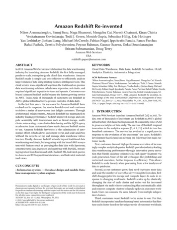
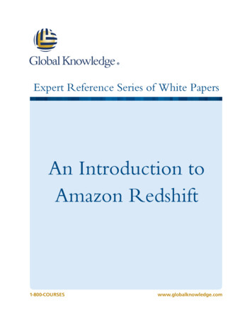
Figure 1: Amazon Redshift ArchitectureRedshift automated workload management, physical tuning, andthe refresh of materialized views (MVs), along with preprocessingthat rewrites queries to use MVs.Fourth, customers expect Redshift to integrate seamlessly withthe AWS ecosystem and other AWS purpose built services. Redshift provides federated queries to transactional databases (e.g.,DynamoDB [10] and Aurora [22]), Amazon S3 object storage, andthe ML services of Amazon Sagemaker. Through Glue Elastic Views,customers can create Materialized Views in Redshift that are incrementally refreshed on updates of base tables in DynamoDB orAmazon OpenSearch. Redshift also provides ingestion and queryingof semistructured data with the SUPER type and PartiQL [2].The rest of the paper is structured as follows. Section 2 gives anoverview of the system architecture, data organization and queryprocessing ow. It also touches on AQUA, Redshift’s hardwarebased query acceleration layer and Redshift’s advanced query rewriting capabilities. Section 3 describes Redshift Managed Storage(RMS), Redshift’s high-performance transactional storage layer andSection 4 presents Redshift’s compute layer. Details on Redshift’ssmart autonomics are provided in Section 5. Lastly, Section 6 discusses how AWS and Redshift make it easy for their customersto use the best set of services for each use case and seamlesslyintegrate with Redshift’s best-of-class analytics capabilities.2 PERFORMANCE THAT MATTERS2.1 OverviewAmazon Redshift is a column-oriented massively parallel processing data warehouse designed for the cloud [13]. Figure 1 depictsRedshift’s architecture. A Redshift cluster consists of a single coordinator (leader) node, and multiple worker (compute) nodes. Datais stored on Redshift Managed Storage, backed by Amazon S3, andcached in compute nodes on locally-attached SSDs in a compressedcolumn-oriented format. Tables are either replicated on every compute node or partitioned into multiple buckets that are distributedamong all compute nodes. The partitioning can be automaticallyderived by Redshift based on the workload patterns and data characteristics, or, users can explicitly specify the partitioning style asround-robin or hash, based on the table’s distribution key.Amazon Redshift provides a wide range of performance andease-of-use features to enable customers to focus on business problems. Concurrency Scaling allows users to dynamically scale-outin situations where they need more processing power to provideconsistently fast performance for hundreds of concurrent queries.Data Sharing allows customers to securely and easily share datafor read purposes across independent isolated Amazon Redshiftclusters. AQUA is a query acceleration layer that leverages FPGAsto improve performance. Compilation-As-A-Service is a cachingmicroservice for optimized generated code for the various queryfragments executed in the Redshift eet.In addition to accessing Redshift using a JDBC/ODBC connection, customers can also use the Data API to access Redshift fromany web service-based application. The Data API simpli es accessto Redshift by eliminating the need for con guring drivers andmanaging database connections. Instead, customers can run SQLcommands by simply calling a secure API endpoint provided bythe Data API. Today, Data API has been serving millions of querieseach day.Figure 2 illustrates the ow of a query through Redshift. Thequery is received by the leader node 1 and subsequently parsed,rewritten, and optimized 2 . Redshift’s cost-based optimizer includes the cluster’s topology and the cost of data movement between compute nodes in its cost model to select an optimal plan.Planning leverages the underlying distribution keys of participatingtables to avoid unnecessary data movement. For instance, if the
3RedshiftABC210join key in an equi-join matches the underlying distribution keysof both participating tables, then the chosen plan avoids any datamovement by processing the join locally for each data partition 3 .After planning, a workload management (WLM) componentcontrols admission to Redshift’s execution phase. Once admitted,the optimized plan is divided into individual execution units thateither end with a blocking pipeline-breaking operation or returnthe nal result to the user. These units are executed in sequence,each consuming intermediate results of previously executed units.For each unit, Redshift generates highly optimized C code thatinterleaves multiple query operators in a pipeline using one or more(nested) loops, compiles it and ships the binary to compute nodes4 . The columnar data are scanned from locally attached SSDsor hydrated from Redshift Managed Storage 5 . If the executionunit requires exchanging data with other compute nodes over thenetwork, then the execution unit consists of multiple generatedbinaries that exchange data in a pipelined fashion over the network.Each generated binary is scheduled on each compute node tobe executed by a xed number of query processes. Each queryprocess executes the same code on a di erent subset of data. Redshift’s execution engine employs numerous optimizations to improve query performance. To reduce the number of blocks thatneed to be scanned, Redshift evaluates query predicates over zonemaps i.e., small hash tables that contain the min/max values perblock and leverages late materialization. The data that needs tobe scanned after zone-map ltering is chopped into shared workunits, similar to [16, 20], to allow for balanced parallel execution.Scans leverage vectorization and Single Instruction, Multiple Data(SIMD) processing for fast decompression of Redshift’s light-weightcompression formats and for applying predicates e ciently. Bloom lters, created when building hash tables, are applied in the scan tofurther reduce the data volume that has to be processed by downstream query operators. Prefetching is leveraged to utilize hashtables more e ciently.Redshift’s execution model is optimized for the underlying Amazon EC2 Nitro hardware, resulting in industry leading price/performance. Figure 3(a) demonstrates Redshift’s competitive edge whenit comes to price-performance. It compares Amazon Redshift andthree other cloud data warehouses and shows that Amazon Redshiftdelivers up to 3 better price-performance ratio out-of-the-box onuntuned 3TB TPC-DS benchmark1 . After all cloud data warehouses1 Weuse the Cloud DW benchmark [1] based on current TPC-DS and TPC-H benchmarks without any query or data modi cations and compliant with TPC rules andrequirements.3 CN10 CN30 CN100 CN210OOBTunedWorkload(a) Price-Performance comparisonFigure 2: Query ow3Time (hours)Relative Price Performance430TB 100TB 300TBScale1PB(b) Scaling TPC-DS from 30TB to 1PBFigure 3: Price-Performance and Scalabilityare tuned, Amazon Redshift has 1.5 better price performance thanthe second-best cloud data warehouse o ering.Customer data grows rapidly rendering scalability a top priority. Figure 3(b) depicts the total execution time of tuned TPC-DSbenchmark while scaling dataset size and hardware simultaneously.Redshift’s performance remains nearly at for a given ratio of datato hardware, as data volume ranges from 30TB to 1PB. This linearscaling to the petabyte-scale makes it easier, predictable and coste cient for customers to on-board new datasets and workloads.The following sub-sections discuss selected aspects from Redshift’s rewriting/optimization and execution model.2.2Introduction to Redshift Code GenerationRedshift is an analytical database focusing on fast execution ofcomplex queries on large amounts of data. Redshift generates C code speci c to the query plan and the schema being executed. Thegenerated code is then compiled and the binary is shipped to thecompute nodes for execution [12, 15, 17]. Each compiled le, calleda segment, consists of a pipeline of operators, called steps. Eachsegment (and each step within it) is part of the physical query plan.Only the last step of a segment can break the pipeline.1 / / Loop o v e r t h e t u p l e s o f R .2 while ( s c a n s t e p h a s n e x t ( ) ) {3/ / Get n e x t v a l u e f o r R . key .4auto f i e l d 1 f e t c h e r 1 . g e t n e x t ( ) ;5/ / Get n ex t v a l u e f o r R . v a l .6auto f i e l d 2 f e t c h e r 2 . g e t n e x t ( ) ;7/ / Apply p r e d i c a t e R . v a l 5 0 .8if ( f i e l d 2 constant1 ) {9/ / Hash R . k e y and p r o b e t h e h a s h t a b l e .10s i z e t h1 hash ( f i e l d 1 ) & ( h a s h t a b l e 1 s i z e 1 ) ;11f o r ( auto p1 h a s h t a b l e 1 [ h1 ] ; p1 ! n u l l p t r ; p1 p1 n e x t ) {12/ / E v a l u a t e t h e j o i n c o n d i t i o n R . key S . key .13i f ( f i e l d 1 p1 f i e l d 1 ) sum1 f i e l d 2 ;14}15 }16 }Figure 4: Example of generated codeFigure 4 shows a high-level example of the generated C codeon a single node cluster for a simple scan ! join ! aggregatequery: ‘SELECT sum(R.val) FROM R, S WHERE R.key S.keyAND R.val 50’. This segment contains the pipeline that scansbase table R (lines 3-6), applies the lter (line 8), probes the hashtable of S (line 10), and computes the aggregate sum() (line 13).Omitted for simplicity from Figure 4 are segments to build thehash table from table S and a nal segment to combine the partialsums across compute nodes and return the result to the user. The
generated code follows the principle of keeping the working setas close to the CPU as possible to maximize performance. As such,each tuple that is processed by multiple operators in a pipelineis typically kept in CPU registers until the tuple is sent over thenetwork, materialized in main memory or ushed to disk.The main property of this style of code generation is that itavoids any type of interpreted code since all operators for a speci cquery are generated in the code on the y. This is in contrast to thestandard Volcano execution model [11], where each operator is implemented as an iterator and function pointers or virtual functionspick the right operator at each execution step. The code generation model o ers much higher throughput per tuple at the costof latency, derived from having to generate and compile the codespeci c to each query. Section 2.6 explains how Redshift mitigatesthe compilation costs.2.3Vectorized ScansIn Figure 4 lines 4 and 6, function 64C 4GC () returns the nextvalue for the corresponding eld of the base table ' de ned by aunique fetcher. Such functions are inlined instead of virtual but areinherently pull-based rather than push-based since the underlyingstructure of the base table is too complicated to represent in thegenerated code directly. This model is relatively expensive as itretains a lot of state for each column scanned, easily exhaustingthe CPU registers if the query accesses more than a few columns.Moreover, the lter predicate evaluation (line 8) involves branchingthat may incur branch misprediction costs if the selectivity of acertain predicate is close to 50%, stalling the pipeline. Finally, eachfetcher may inline a large amount of decompression code, whichcan signi cantly slow down compilation for wide tables that accessa large number of columns.To address these issues, Redshift added a SIMD-vectorized scanlayer to the generated code that accesses the data blocks and evaluates predicates as function calls. In contrast to the rest of the stepsthat compile the code on the y, the vectorized scan functions areprecompiled and cover all data types and their supported encodingand compression schemes. The output of this layer stores the column values of the tuples that qualify from the predicates to localarrays on the stack accessed by downstream steps. In addition to thefaster scan code due to SIMD, this reduces the register pressure andthe amount of inline code that must be compiled, leading to ordersof magnitude faster compilation for certain queries on wide tables.The design combines column-at-a-time execution for a chunk oftuples during the scan step and tuple-at-a-time execution downstream for joins and aggregation steps. The size of the chunk that isprocessed column-at-a-time is dynamically determined during codegeneration based on the total width of the columns being accessedand the size of the thread-private (L2) CPU cache.2.4Reducing Memory Stalls with PrefetchingRedshift’s pipelined execution avoids the materialization of intermediate results for the outer stream of joins and aggregates bykeeping the intermediate column values in CPU registers. However,when building or probing hash tables as part of a hash join, orprobing and updating hash tables as part of aggregations, Redshiftincurs the full overhead of a cache miss if the hash table is toolarge to t in the CPU cache. Memory stalls are prominent in thispush-based model and may o set the eliminated cost of materialization for the outer stream in joins. The alternative would be topartition the input until the hash table of the partition ts in theCPU cache, thus avoiding any cache misses. That model, however,is infeasible for the execution engine since it may not be able toload large base tables in memory and thus cannot access payloadcolumns using record identi ers. Instead, Redshift transfers all theneeded columns downstream across the steps in the pipeline andincurs the latency of a cache miss when the hash table is largerthan the CPU cache.Since cache misses are an inherent property of our execution engine design, stalls are mitigated using prefetching. Our prefetchingmechanism is integrated in the generated code and interleaves eachprobe in the hash table or Bloom lter with a prefetch instruction.Redshift keeps a circular bu er in the fastest (L1) CPU cache and,for each tuple that arrives, prefetches and pushes it in the bu er.Then, an earlier tuple is popped and pushed downstream to therest of the steps. Once the bu er is lled up, rather than bu eringmultiple tuples, individual tuples are processed by pushing andpopping one at a time from the bu er.This model trades some materialization cost to the cache-residentprefetching bu er for the bene t of prefetching the hash tableaccesses and reducing the memory stalls. We have found this tradeo to always be bene cial if the hash table is larger than the CPUcache. If the hash table is known or expected to be small enoughto t in the CPU cache, this additional code is never generated.The same happens if the tuple is too wide and storing it in thebu er would be more expensive than paying for the cache missstall. On the other hand, the prefetching code may be generatedmultiple times in the same nested loop if there are multiple joinsand group-by aggregation in the same pipeline, while ensuring thatthe total size of all prefetching bu ers is small enough to remain inthe fastest (L1) CPU cache.2.5Inline Expression FunctionsWhile the examples above cover basic cases of joins and aggregations with simple data types, an industrial-grade database needsto support complex data types and expression functions. The generated code includes pre-compiled headers with inline functionsfor all basic operations, like hashing and string comparisons. Scalarfunctions that appear in a query translate to inline or regular function calls in the generated code, depending on the complexity of thequery. Most of these functions are scalar, as they process a singletuple, but may also be SIMD-vectorized internally.In Redshift, most string functions are vectorized with SIMDcode tailored to that particular function. One such example are theLIKE predicates that use the pcmpestri instruction in Intel CPUs,which allows sub-string matching of up to 16-byte patterns in asingle instruction. Similarly, functions such as UPPER(), LOWER(),and case-insensitive string comparisons, use SIMD code to accelerate the ASCII path and only fall back to (optimized) scalar codewhen needed to handle more complex Unicode characters. Suchoptimizations are ubiquitous in expression functions to maximizethroughput. The code generation layer inlines function calls thatare on the critical path when advantageous.
2.6Compilation ServiceWhen a query is sent to Redshift, the query processing engine compiles optimized object les that are used for query execution. Whenthe same or similar queries are executed, the compiled segmentsare reused from the cluster code compilation cache, which resultsin faster run times because there is no compilation overhead. WhileRedshift minimizes the overhead of query compilation, the very rst set of query segments still incurs additional latency. In somecases, even a small additional latency can impact a mission criticalworkload with tight service-level-agreements (SLAs), particularlywhen a large number of segments need to be compiled increasingcontention for cluster resources.The compilation service uses compute and memory resourcesbeyond the Redshift cluster to accelerate query compilation througha scalable and secure architecture. The compilation service cachesthe compiled objects o -cluster in an external code cache to servemultiple compute clusters that may need the same query segment.During query processing, Redshift generates query segments andleverages the parallelism of the external compilation service forany segments that are not present in a cluster’s local cache or theexternal code cache. With the release of compilation service cachehits across the Amazon Redshift eet have increased from 99.60%to 99.95%. In particular, in 87% of the times that an object le wasnot present in a cluster’s local code cache, Redshift found it in theexternal code cache.2.7CPU-Friendly EncodingPerformance is closely tied to CPU and disk usage. Naturally, Redshift uses compression to store columns on disk. Redshift supportsgeneric byte-oriented compression algorithms such as LZO andZSTD, as well as optimized type-speci c algorithms. One such compression scheme is the recent AZ64 algorithm, which covers numericand date/time data types. AZ64 achieves compression that is comparable to ZSTD (which compresses better than LZO but is slightlyslower) but with faster decompression rate. For example, a full 3TBTPC-H run improves by 42% when we use AZ64 instead of LZO forall data types that AZ64 supports.2.8Adaptive ExecutionRedshift’s execution engine takes runtime decisions to boost performance by changing the generated code or runtime properties on the y based on execution statistics. For instance, the implementationof Bloom lters (BFs) in Redshift demonstrates the importance ofdynamic optimizations [6]. When complex queries join large tables,massive amounts of data might be transferred over the network forthe join processing on the compute nodes and/or might be spilledto disk due to limited memory. This can cause network and/orI/O bottlenecks that can impact query performance. Redshift usesBFs to improve the performance of such joins. BFs e ciently lterrows at the source that do not match the join relation, reducing theamount of data transferred over the network or spilled to disk.At runtime, join operations decide the amount of memory thatwill be used to build a BF based on the exact amount of data thathas been processed. For example, if a join spills data to disk, thenthe join operator can decide to build a larger BF to achieve lowerfalse-positive rates. This decision increases BFs pruning power andmay reduce spilling in the probing phase. Similarly, the enginemonitors the e ectiveness of each BF at runtime and disables itwhen the rejection ratio is low since the lter burdens performance.The execution engine can re-enable a BF periodically since temporalpattern of data may render a previously ine ective BF to becomee ective.2.9AQUA for Amazon RedshiftAdvanced Query Accelerator (AQUA) is a multi-tenant service thatacts as an o -cluster caching layer for Redshift Managed Storageand a push-down accelerator for complex scans and aggregations.AQUA caches hot data for clusters on local SSDs, avoiding the latency of pulling data from a regional service like Amazon S3 andreducing the need to hydrate the cache storage in Redshift compute nodes. To avoid introducing a network bottleneck, the serviceprovides a functional interface, not a storage interface. Redshiftidenti es applicable scan and aggregation operations and pushesthem to AQUA, which processes them against the cached data andreturns the results. Essentially, AQUA is computational storage at adata-center scale. By being multi-tenant, AQUA makes e cient useof expensive resources, like SSDs, and provides a caching servicethat is una ected by cluster transformations such as resize andpause-and-resume.To make AQUA as fast as possible, we designed custom serversthat make use of AWS’s Nitro ASICs for hardware-accelerated compression and encryption, and leverage FPGAs for high-throughputexecution of ltering and aggregation operations. The FPGAs arenot programmed on a per-query basis, but rather used to implement a custom multi-core VLIW processor that contains databasetypes and operations as pipelined primitives. A compiler withineach node of the service maps operations to either the local CPUsor the accelerators. Doing this provides signi cant acceleration forcomplex operations that can be e ciently performed on the FPGA.2.10Query Rewriting FrameworkRedshift features a novel DSL-based Query Rewriting Framework(QRF), which serves multiple purposes: First, it enables rapid introduction of novel rewritings and optimizations so that Redshift canquickly respond to customer needs. In particular, QRF has been usedto introduce rewriting rules that optimize the order of executionbetween unions, joins and aggregations. Furthermore, it is usedduring query decorrelation, which is essential in Redshift, whoseexecution model bene ts from large scale joins rather than bruteforce repeated execution of subqueries.Second, QRF is used for creating scripts for incremental materialized view maintenance (see Section 5.4) and enabling answering queries using materialized views. The key intuition behindQRF is that rewritings are easily expressed as pairs of a patternmatcher, which matches and extracts parts of the query representation (AST or algebra), and a generator that creates the new queryrepresentation using the parts extracted by the pattern matcher.The conceptual simplicity of QRF has enabled even interns to develop complex decorrelation rewritings within days. Furthermore,it enabled Redshift to introduce rewritings pertaining to nested andsemistructured data processing (see Section 6.4) and sped up theexpansion of the materialized views scope.
3SCALING STORAGEThe storage layer of Amazon Redshift spans from memory, to localstorage, to cloud object storage (Amazon S3) and encompasses allthe data lifecycle operations (i.e., commit, caching, prefetching,snapshot/restore, replication, and disaster-recovery). Storage hasgone through a methodical and carefully deployed transformationto ensure durability, availability, scalability, and performance:Durability and Availability. The storage layer builds on AmazonS3 and persists all data to Amazon S3 with every commit. Buildingon Amazon S3 allows Redshift to decouple data from the computecluster that operates on the data. It also makes the data durable andbuilding an architecture on top of it enhances availability.Scalability. Using Amazon S3 as the base gives virtually unlimited scale. Redshift Managed Storage (RMS) takes advantage ofoptimizations such as data block temperature, data block age, andworkload patterns to optimize performance and manage data placement across tiers of storage automatically.Performance. Storage layer extends into memory and algorithmicoptimizations. It dynamically prefetches and sizes the in-memorycache, and optimizes the commit protocol to be incremental.3.1Redshift Managed StorageThe Redshift managed storage layer (RMS) is designed for a durability of 99.999999999% and 99.99% availability over a given year,across multiple availability zones (AZs). RMS manages both userdata as well as transaction metadata. RMS builds on top of the AWSNitro System, which features high bandwidth networking and performance indistinguishable from bare metal. Compute nodes uselarge, high performance SSDs as local caches. Redshift leveragesworkload patterns and techniques such as automatic ne-graineddata eviction and intelligent data prefetching, to deliver the performance of local SSD while scaling storage automatically to AmazonS3.Figure 5 shows the key components of RMS extending from inmemory caches to c
data warehousing solutions, which were expensive, not elastic, and required signi cant expertise to tune and operate. Customers em- . Amazon Redshift is a column-oriented massively parallel process-ing data warehouse designed for the cloud [13]. Figure 1 depicts Redshift's architecture. A Redshift cluster consists of a single coor-
![Index [beckassets.blob.core.windows ]](/img/66/30639857-1119689333-14.jpg)