Transcription
Noname manuscript No.(will be inserted by the editor)Extensions to the Design Structure Matrix for the Description ofMultidisciplinary Design, Analysis, and Optimization ProcessesAndrew B. Lambe · Joaquim R. R. A. MartinsReceived: date / Accepted: dateAbstract While numerous architectures exist for solvingmultidisciplinary design optimization (MDO) problems, thereis currently no standard way of describing these architectures. In particular, a standard visual representation of thesolution process would be particularly useful as a communication medium among practitioners and those new to thefield. This paper presents the extended design structure matrix (XDSM), a new diagram for visualizing MDO processes.The diagram is based on extending the standard design structure matrix (DSM) to simultaneously show data dependencyand process flow on a single diagram. Modifications includeadding special components to define iterative processes, defining different line styles to show data and process connections independently, and adding a numbering scheme to define the order in which the components are executed. Thispaper describes the rules for constructing XDSMs along withmany examples, including diagrams of several MDO architectures. Finally, this paper discusses potential applicationsof the XDSM in other areas of MDO and the future development of the diagrams.This work was presented by the authors under the title “A UnifiedDescription of MDO Architectures” at the 9th World Congress onStructural and Multidisciplinary Optimization. This work was partiallyfunded by a postgraduate scholarship from the Natural Sciences andEngineering Research Council of Canada.A. B. LambeInstitute for Aerospace StudiesUniversity of TorontoToronto, Ontario, CanadaE-mail: lambe@utias.utoronto.caJ. R. R. A. MartinsDepartment of Aerospace EngineeringUniversity of MichiganAnn Arbor, Michigan, USAE-mail: jrram@umich.eduKeywords Multidisciplinary Design Optimization · Visualization · Design Structure Matrix · Design Architectures ·Multidisciplinary Analysis · Distributed Optimization1 IntroductionWhen employing multidisciplinary design optimization (MDO)to solve a given design problem, designers are confrontedwith a wide range of options. For example, should the optimizer interact with the analysis software in a “black-box”fashion or should the governing equations be provided to theoptimizer directly? Should a surrogate model be employed?Which disciplines or system components should be resolvedin a coupled fashion? Should decomposition be employedin the optimization problem? Should the decomposition employ a penalty function scheme or a multilevel scheme? Inpractice, these kinds of questions are answered on a caseby-case basis after considering the problem characteristics,distribution of expertise, level of communication betweendesigners, and available software tools. However, the answers to these questions strongly influence both the optimization problem formulation and the solution strategy employed which, in turn, strongly influence the time and resources needed to find a design solution.We refer to the combination of the design problem formulation and the organizational framework used to solve itas an MDO architecture. Many architectures have been developed, including multidisciplinary feasible (MDF) (Crameret al, 1994), individual discipline feasible (IDF) (Crameret al, 1994), concurrent subspace optimization (CSSO) andits variants (Bloebaum et al, 1992; Sellar et al, 1996; Wujeket al, 1996), collaborative optimization (CO) and its variants(Braun and Kroo, 1997; Kroo, 1997; DeMiguel and Murray, 2000; Roth, 2008), bilevel integrated system synthesis (BLISS) and its variants (Sobieszczanski-Sobieski et al,
22000, 2003; Kodiyalam and Sobieszczanski-Sobieski, 2000),and analytical target cascading and its variants (Kim, 2001;Kim et al, 2003, 2006; Tosserams et al, 2006). Determiningthe conditions under which each architecture is most effective and refining their performance remains an active area ofresearch.Once an architecture has been selected, it must be implemented in the computational environment. As with othercomputational methods, incorrect implementation of the MDOarchitecture can prevent solution of the design problem. However, determining the correct implementation can be difficultbecause there is no standard way of describing the solutionprocess. Each author uses his/her own notational set, algorithmic description, and system of diagrams in describinga new architecture. The lack of a standard representation ofMDO architectures is a barrier to communicating the correctimplementation and describing alternative approaches.This work is complementary to a number of other studies in the MDO literature that seek more flexible ways of describing MDO problems and solution methods. Alexandrovand Lewis (2004a,b) proposed a linguistic approach to problem formulation called reconfigurable multidisciplinary synthesis (REMS). The REMS framework used a small set ofcomputational components along with a directed graph representation to allow the user to quickly reformulate a specified MDO problem. Later work by Tosserams et al (2010)created the Ψ language to allow the user greater freedom inthe assembly of the problem formulation, especially for decomposed problems. Another language, called χ, was created by Etman et al (2005) to specify the coordination strategy for parallel solution processes. While linguistic approacheslike these are useful for automatically implementing MDOarchitectures in a computational environment (Martins et al,2009), they do not provide a formal visual representation ofhow the architecture handles the original problem.Our work is most similar to the work of De Wit and VanKeulen (2010), who present a unified set of mathematicalnotation and diagrams to describe a broad range of decomposition and coordination strategies. Unlike the linguisticapproaches mentioned above, the diagrams provide a visualframework for describing MDO architectures. However, inthat work, multiple diagrams are required to explain the decomposition and coordination strategies employed. We feelthat a similar approach using only one diagram would bea more accessible starting point, facilitating communicationabout MDO architectures among experts and nonexperts alike.In this work, we present our approach to the problem ofcreating a standard visual representation of the solution process of an MDO architecture. While this paper is focused onMDO architectures in particular, we have found that our diagram syntax may be more broadly applicable to a range ofanalysis and optimization processes. Indeed, we should expect this, given the commonality in the computational com-Andrew B. Lambe, Joaquim R. R. A. Martinsponents between the processes. We also integrate mathematical notation into the diagrams and show links between theelements of the diagram and the underlying mathematics.We refer to our diagram as an extended design structure matrix, or XDSM.This paper is organized as follows. Section 2 introducesthe mathematical notation and reviews basic MDO terminology. Section 3 discusses the guiding design principlesand evaluates alternative diagrams for their use in describingMDO processes. Section 4 outlines the elements and syntaxof the XDSM with simple examples. Section 5 shows fourdifferent MDO architectures represented using XDSMs. Section 6 discusses potential applications of the XDSM beyondMDO architectures. Finally, Section 7 provides concludingremarks.2 Terminology and NotationBefore discussing the diagrams themselves, we introducethe notation that is used throughout this paper. This notation was developed to compare the various problem formulations within MDO architectures and is listed in Table 1.This is not a comprehensive list; additional notation specificto particular architectures is introduced when the respectivearchitectures are described. We also take this opportunity toclarify many of the terms we use that are specific to the fieldof MDO.A design variable is a variable in the MDO problem thatis always under the explicit control of an optimizer. Designvariables may pertain to a single discipline, i.e., be local, ormay be shared by multiple disciplines. We denote the vectorof design variables local to discipline i by xi and the sharedvariables by x0 . The full vector of design variables is given Tby x xT0 , xT1 , . . . , xTN . The subscripts for local and shareddata are also used in describing objectives and constraints.A discipline analysis is a simulation that models the behavior of one aspect of a multidisciplinary system. Conducting a discipline analysis consists of solving a systemof equations and returning a set of response variables. Theresponse variables may or may not be controlled by the optimization, depending on the formulation. We denote thevector of response variables computed within discipline iby yi . Analogously to the design variables, the full vectorof response variables is denoted y. In a multidisciplinarysystem, most disciplines are required to exchange their response variables with other disciplines to model the interactions of the whole system. Often, the number of variables exchanged is much smaller than the total number of responsevariables computed in a particular discipline. Those variables that are exchanged are referred to as coupling variables.
Extensions to the Design Structure Matrix3Table 1 Mathematical notation for MDO problem dataSymbolDefinitionxytyfcccN()0()i() ()Vector of design variablesVector of coupling variable targets (inputs to a discipline analysis)Vector of coupling variable responses (outputs from a discipline analysis)Objective functionVector of design constraintsVector of consistency constraintsNumber of disciplinesFunctions or variables that are shared by more than one disciplineFunctions or variables that apply only to discipline iFunctions or variables at their optimal valueApproximation of a given function or vector of functionsIn many formulations, copies of the coupling variablesmust be made to allow discipline analyses or optimizationsto run independently and in parallel. These copies are knownas target variables and are denoted by a superscript t. Forexample, the copy of the response variables produced bydiscipline i is denoted yti . These variables are used as theinput to disciplines other than discipline i that are coupledto discipline i through yi . To preserve consistency betweenthe coupling variable inputs and outputs at the optimal solution, we define a set of consistency constraints, cci yti yi ,that we add to the problem formulation. (These constraintsare sometimes referred to as compatibility constraints. However, we use the term consistency to avoid confusion with thecompatibility constraints present in structural analysis.)Each of these elements of the MDO problem is handleddifferently in different architectures. Several of the problemformulations are discussed in Section 5 along with their corresponding XDSMs.3 Design PrinciplesWe now return to the primary objective of this paper: developing a standard visual representation of an MDO solutionprocess. In particular, we want to capture the basic algorithmand all the data connections in a single diagram. We basedthe graphic design on the following guiding principles:1. Simplicity. MDO processes can be complex because ofthe number of different analysis codes needed to model acoupled system and the volume and varied types of datathat these codes exchange. In spite of this complexity,the diagram syntax should have as few rules and symbolsas possible to make the description of the process clear.We expect the average user to understand the syntax wellenough that they can create their own diagrams after anhour of study.2. Clarity. The depiction of the data exchange and algorithm should have an unambiguous meaning to the viewer.We are particularly concerned with the reproducibility ofthe depicted processes and avoiding errors in communication. This is especially important in explaining MDOprocesses to nonspecialists and those new to the field.3. Information Density. Because MDO processes involvemany computational elements exchanging data withinan overall algorithm, we wish to depict both the algorithm and the data exchanges simultaneously. Incorporating data and process into a single diagram gives usan immediate impression of the whole software architecture without having to compare and cross-check multiple diagrams.4. Integration of Mathematics. Because MDO processes incorporate many mathematical representations in the formof systems of equations, optimization problem statements,inequalities defining convergence conditions, etc., the diagram should be able to incorporate the notation wherepossible to enhance understanding. This should be doneso long as it does not interfere with the other principlesoutlined above. If the mathematics cannot be incorporated into the diagram directly, the locations of the relevant expressions should be obvious to the viewer. Usingmathematics directly in the diagram also helps to compact the data into a small space without loss of information (Tufte, 1983).Using these principles, we now review some commonly useddiagrams in the MDO and complex system literature.The first diagram we review is the standard flowchart.Flowcharts depict algorithms by representing simple operations (selection, initialization, input and output, etc.) bydifferent block shapes connected by lines. Flowcharts canalso be scaled to show large, complex algorithms. Whilethese diagrams are simple to understand and have been usedsuccessfully for many years, they do not track data movement among the computer program components. Because ofthe nature of the MDO computing environment, with manycomputational elements exchanging data at key points in thealgorithm, some representation of the data transfer is alsonecessary. Separate data flow diagrams may be employed
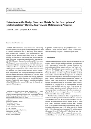
4but, as mentioned above, we prefer to use a single diagram.Adding data transfer lines to a flowchart is another possibility. However, the number of lines required in complex architectures could turn the diagram into “spaghetti” and make ithard to interpret.A common visualization technique used in the MDO literature is some type of block diagram (Braun et al, 1996;Sobieszczanski-Sobieski et al, 2000; Perez et al, 2004). Typically, these diagrams use blocks to represent computationalcomponents and labeled arrows to show data flow. These diagrams suffer from the opposite problem of the flowchart:they show the data exchange well but do not clearly define the process. This is especially true when multiple loopsare present in the algorithm or when certain components arereused within a loop. Another consideration is that there isno standard way of constructing the block diagram, so eachdiagram must be interpreted individually.Another option for visualization is the unified modelinglanguage (UML) (Booch et al, 2005). UML was designedto model and visualize software systems, especially objectoriented software, under a unified standard. (An exampleof UML class diagrams is given by Martins et al (2009).)Because of the close connections between object-orientedsoftware and MDO (Alexandrov and Lewis, 2004a,b), wemay expect that the same visualization tools can be used inboth cases. In contrast to the other methods that we havedescribed, UML is standardized, and this adds to its appeal for widespread communication. However, describingan MDO process using UML would require multiple diagrams to show both the process and data flows, a situationthat we want to avoid. We also feel that UML is difficultto learn, and this is an additional barrier to communicationabout MDO.Finally, a diagram that is common in systems engineering is the N2 diagram (Lano, 1977) or design structure matrix (DSM) (Steward, 1981). An example DSM for an aircraft design problem is shown in Fig. 1. While several different types of DSM exist (Browning, 2001), the basic diagram is unchanged. The components of a system are placedon the main diagonal of a matrix with the inputs to eachcomponent placed in the same column and the outputs fromeach component placed in the same row. External inputsand outputs, if they are considered, are placed on the outside edges of the diagram. The key advantage of DSM is astrict diagram structure. Whereas traditional block diagramsand flowcharts allow the system components and interconnections to be placed arbitrarily, the DSM structure effectively “untangles” the collection of components and givesthe reader a complete view of the coupling structure withinthe system. The DSM in Fig. 1 further enhances this viewby using larger dots to denote stronger coupling betweenthe disciplines. Other notation may be used to show morecoupling information, e.g., see Yassine and Braha (2003).Andrew B. Lambe, Joaquim R. R. A. MartinsAOptimization AAerodynamics stemOGHIJKLM NOBCDEPerformance HSizingFAFGHIJKLMNOFig. 1 Example DSM for aircraft design problem.The principal disadvantage of the DSM lies in the definition of the order of execution of the components. Whilesome DSMs show a sequence by ordering the componentsalong the diagonal of the matrix (Browning, 2001), we require more flexibility in the ordering because of the selection, iteration, and parallel computing structures present inMDO architectures. These structures can be considered ahigh-level algorithm driving the architecture. Furthermore,we would like to maintain the property of the standard DSMthat a reordering of the components does not change theunderlying system. Therefore, we have chosen to add additional graphical features to the DSM to show process flowsat the same time as data flows. These features are describedin detail in the next section.4 XDSM Syntax DescriptionAs explained above, the DSM structure offers a convenientand compact way to represent the connections between system components. When the DSM is applied to the specificcase of a computational MDO environment, the componentsof the system are computational elements (disciplinary analyses, optimizers, surrogate models, etc.), and the connections consist of the data passed between them. However, forprocesses, such as the algorithms of MDO architectures, werequire the diagram to show the order in which the components are executed without ordering the components. Furthermore, we need a way to show iterative procedures on thediagram. This section describes the extensions necessary tocreate an XDSM from a DSM.(All XDSMs shown in this work were created in LaTeXusing the TikZ package. To simplify the diagram creation,we have developed template files containing all necessaryblock shapes and line styles. These templates and some ex-
Extensions to the Design Structure MatrixAnalysis 1y25y1y2Analysis 2y3y3ytx0 , x1x0 , x2x0 , x3(no data)0,2 1:MDA1 : y2t , y3t1 : y1t , y3t1 : y1t , y2ty12 : y11:Analysis 1y22 : y2y32 : y3y1Analysis 31:Analysis 21:Analysis 3Fig. 4 Jacobi MDA procedure with parallel execution of components.Fig. 2 Generic, three-discipline, fully coupled system.tion is to distribute the state target information appropriatelyand to check the convergence of the MDA process. We re0,4 1:(no data)1 : y2t , y3t2 : y3tfer to the components controlling an iterative procedure asMDAdrivers. We use a separate shape (a rounded rectangle, in this1:y14 : y12 : y13 : y1case) to distinguish drivers from other components.Analysis 1The order in which the components are executed is de2:y24 : y23 : y2fined by numbering the components, starting at zero. TheAnalysis 2components are executed in numerical order unless a loop is3:y34 : y3present. A loop is denoted by m n, where n m. This noAnalysis 3tation means that before proceeding to m 1, the sequencereturns to component n until the condition defined by theFig. 3 Gauss–Seidel MDA procedure.driver is satisfied. The data blocks are also numbered to clarify the step at which the data are passed to the component.This is useful in more complicated diagrams where the sameample XDSM source code are freely available for downloadcomponent takes input from different sources at differentat w.steps. (The BLISS-2000 architecture depicted in Fig. 12 is aComments and suggestions are welcome.)good example of this.) Finally, to give an added visual cueWe start with the task of performing a multidisciplinaryto the process flow, we use a distinct line style to connectanalysis (MDA) on a coupled system with three disciplines.consecutive components. In our XDSMs, a thick gray lineAn MDA is an iterative process that computes a set of courepresents data connections, while a thin black line reprepling variables that satisfies the consistency constraints ofsents process connections. These line styles were chosen soa coupled system. Figure 2 shows the original DSM for thisthat they could coexist on the diagram, i.e., so that one doessystem. In this diagram, we have used different block shapesnot overwrite the other.to distinguish between the computational analyses and theThe same MDA can be solved using other types of itdata connections. The shapes were chosen for their similarerations, such as Jacobi iterations. Figure 4 shows a Jacobiity with flowchart syntax: rectangles for generic processes,iteration, where all the analysis components are executed usparallelograms for data input and output. The data depening the state information from the previous Jacobi iteration.dency of the components is further emphasized by the useTo show that each of these components may be executed inof thick gray lines to connect the nodes.parallel, we use the same number for each component. NoteIn a Gauss–Seidel MDA process, each analysis is exethat no data are exchanged between these components durcuted in sequence using a set of design variables (chosening the parallel execution. If it is not possible to evaluate theoutside the MDA) and the most recent information on thediscipline analyses in parallel, we can also use the XDSMstates of the other disciplines. The analyses continue untilto capture sequential execution. A Jacobi iteration with sea consistent set of state variables is returned by the individquentially executed components is depicted in Fig. 5.ual disciplines. These states are then returned to the user orBecause the situation in Fig. 4 of many similar composome external process. Figure 3 shows the XDSM for thenents being executed in parallel occurs frequently in MDO,Gauss–Seidel MDA.we have adopted a special convention to make the diagrammore compact. The convention is that a reference to comWe now address the new elements that we have introponent i implies that the diagram structure is repeated forduced to create an XDSM. To control the iteration we haveintroduced a special component, labeled “MDA,” whose func- all disciplines. As an example, Fig. 6 is identical to Fig. 4,ytx0 , x1x0 , x2x0 , x3
6Andrew B. Lambe, Joaquim R. R. A. Martinsytx0 , x1x0 , x2x0 , x30,4 1:MDA1 : y2t , y3t2 : y1t , y3t3 : y1t , y2ty14 : y11:Analysis 1y24 : y2y34 : y3(no data)x 2:Analysis 23:Analysis 3Fig. 5 Jacobi MDA procedure with sequential execution of components.yt(no data)yix(0)0,2 1:MDA2 : yi2:f1:Objective1:Constraintsx(0)0,2 1:Optimization1:x2:f1:Objective1:Analysis i2:cFig. 6 Jacobi MDA procedure with parallel execution of componentsusing our convention for parallel diagram structure. Process shownhere is identical to that shown in Fig. 4.1:xFig. 7 Simple optimization algorithm.x 1:1:x2:cx0 , xiyj6t i0,2 1:Optimization2 : df / dx, dc/ dx1:x1:x1:Constraints1:GradientsFig. 8 Optimization algorithm where optimizer requires gradient information. Gradients are calculated by separate component.except that it applies this convention. The presence of theAnalysis i block in Fig. 6 implies that all the disciplinaryanalyses are evaluated in parallel before the algorithm continues. This convention is further enhanced by showing stacksof component and data blocks.Using our syntax, we can also describe optimization processes. Figure 7 shows the solution of a standard nonlinearprogramming problem. An initial guess of the design variables, x(0) , is passed to the optimizer. In each iteration, theobjective and constraints are evaluated, (in parallel, in thiscase,) and an updated set of design variables is computed.The iterations continue until the optimization driver converges, returning the optimal solution x . Note that Fig. 7is independent of the type of optimizer used, i.e., it is independent of the specific calculations that take place within theoptimization driver. If the optimizer also required the gradients of the objective and constraint functions, these couldbe placed in the diagram as additional components with theappropriate connections to the optimization driver. Figure 8shows an optimization algorithm with a separate componentthat computes all the gradient information required by theoptimizer.To conclude this section, we make a few remarks onthe relationship between the XDSMs we have constructedand the underlying mathematics of the MDA and optimization processes. The key point is that, in all of our diagrams,each component corresponds to a set of mathematical ex-pressions, and entry into each component corresponds to theevaluation of these expressions. For example, evaluating the“Constraints” component in Fig. 7 or 8 is the same as computing the values of all the constraint functions in the nonlinear programming problem. The “MDA” and “Optimization”drivers evaluate expressions that compute the next point totest in the iteration. The stopping criterion for the iterationis also checked by the driver. We emphasize that this interpretation extends to all components in all XDSMs, closelylinking the mathematics of the MDO problems to the XDSMdescription of the solution process.5 MDO Architecture ExamplesWe now have all the tools needed to provide a complete description of an MDO architecture. We describe only a fewarchitectures in detail here. However, we note that we havebeen able to describe a total of fifteen general architecturesusing the XDSM, all of which will be presented in detail ina forthcoming survey paper.In the multidisciplinary feasible (MDF) architecture (Crameret al, 1994), all the disciplines are coupled together, and anMDA is performed to compute the full set of state variablesfor a given choice of design variables. MDF is effectively an
Extensions to the Design Structure Matrix7y t,(0)x(0)x 0, 7 1:Optimization2 : x0 , x13 : x0 , x24 : x0 , x36:x1, 5 2:MDA2 : y2t , y3t3 : y3ty1 5 : y12:Analysis 13 : y14 : y16 : y1y2 5 : y23:Analysis 24 : y26 : y2y3 5 : y34:Analysis 36 : y36:Functions7 : f, cFig. 9 Multidisciplinary feasible (MDF) architecture.extension of a single-discipline optimization to the multiplediscipline case, where the MDA replaces a single-disciplineanalysis. The optimization problem formed in this architecture is given bymin.f0 (x, y (x))w.r.t. xs.t.c0 (x, y (x)) 0ci x0 , xi , yi x0 , xi , y j6 i(1) 0i 1, . . . , N.Note the functional notation. Objective f0 is a function ofboth the design variables x and state variables y. Because ofthe MDA process, the state variables are themselves functions of x.Figure 9 shows the XDSM for MDF, using the Gauss–Seidel MDA shown in Fig. 3. The sequence of operationscan be inferred from Fig. 9 following the numbering rulesdefined previously. The operations corresponding to eachnumber in the diagram are as follows:0.1.2.3.4.5.Pass initial data to Optimization and MDA drivers.Initiate MDA.Evaluate Analysis 1.Evaluate Analysis 2.Evaluate Analysis 3.Check MDA convergence. If it has not converged, returnto 2; otherwise, continue.6. Compute objective and constraint function values.7. Compute new design point. If optimization has not converged, return to 1; otherwise, return optimal solution.Note that we have not chosen the convergence criteria of theMDA or the optimization, but we have specified where theseconvergence criteria are applied. These criteria can be chosen by the user and assigned to the corresponding architecture loop. There is also flexibility in the choice of optimizerand multidisciplinary analysis method; we need not use theGauss–Seidel strategy shown in Fig. 9. If, for example, aJacobi or Newton-like strategy is available, it may be substituted into the architecture. For the purpose of this work, wehave tried to keep the description of both problem and solution strategy as generic as possible. Specific implementationdetails are left to the user, but all can be described with anXDSM without difficulty.In the individual discipline feasible (IDF) architecture(Cramer et al, 1994), individual disciplines are not coupledtogether in the analysis of the system. Instead, coupling variable targets are used to share information between disciplines, and consistency constraints are used in the optimization problem to ensure that the coupling variable inputs matchthe disciplinary outputs at the optimal solution. The resulting optimization problem is given bymin.f0 x, y x, ytw.r.t.x, yts.t. c0 x, y x, yt 0 ci x0 , xi , yi x0 , xi , ytj6 i 0 cci yti yi x0 , xi , ytj6 i 0(2)i 1, . . . , Ni 1, . . . , N.Note that the coupling variable outputs, y, are treated asfunctions of design variables and coupling variable inputs,yt , because each iteration of the method involves the evaluation of each discipline analysis. Therefore, coupling vari-
8Andrew B. Lambe, Joaquim R. R. A. Martinsx(0) , y t,(0)x 0,3 1:Optimizationyi 1 : x0 , xi , yj6t i2 : x, y t1:Analysis i2 : yi2:Functions3 : f, c, ccFig. 10 Individual discipline feasible (IDF) architecture.able outputs may take only values that satisfy the governingequations of each discipline.Figure 10 shows the XDSM for IDF.
Keywords Multidisciplinary Design Optimization Visu-alization Design Structure Matrix Design Architectures Multidisciplinary Analysis Distributed Optimization 1 Introduction When employing multidisciplinary design optimization (MDO) to solve a given design problem, designers are confronted with a wide range of options. For example, should the op-