Transcription
Differential Equationsin Finance and Life InsuranceMogens Steffensen1IntroductionThe mathematics of finance and the mathematics of life insurance were always intersecting.Life insurance contracts specify an exchange of streams of payments between the insurancecompany and the contract holder. These payment streams may cover the life time of the contractholder. Therefore, time valuation of money is crucial for any measurement of payments due in thepast as well as in the future. Life insurance companies never put their money under the pillow, andaccumulation and distribution of capital gains were always part of the insurance business. Withrespect to the future, appropriate discounting of contractual obligations qualifies the estimates ofliabilities.Financial contracts specify an exchange of streams of payments as well. However, while thelife insurance payment stream is partly linked to the state of health of the insured, the financialpayment stream is linked to the ’state of health’ of an enterprise. That could be the stream ofdividends distributed to the owners of the enterprise or the stream of claims contingent on the priceof the enterprise paid to the holder of a so-called derivative. The discipline of personal finance isparticularly closely linked to life insurance. Decisions on e.g. consumption, investment, retirement,and insurance coverage belong to some of the most substantial life time financial decisions of anindividual.Valuation of payment streams is probably the most important discipline in the intersectionbetween finance and life insurance. Various valuation dogmas are in play here. The principle ofno arbitrage and the market efficiency assumption are taken as given in the majority of modernacademic approaches to valuation of financial contracts. Life insurance contract valuation typicallyrelies on independence, or at least asymptotic independence, between insured lives. Then the lawof large numbers ensures that reasonable estimates can be found if the portfolio of insurancecontracts is sufficiently large. Both dogmas reduce the valuation problem to being primarily amatter of calculation of conditional expected values.Conditional expected values can be approached by several different techniques. E.g. MonteCarlo simulation exploits that conditional expected values can be approximated by empiricalmeans. Sometimes, however, one can go at least part of the way by explicit calculations. E.g.if a series of auxiliary models with explicit expected values converges towards the real model insuch a way that the series of explicit expected values converges to the desired quantity. A differentroute can be taken when the underlying stochastic system is Markovian, i.e. if given the presentstate, the future is independent of the past. Then solutions to certain systems of deterministicdifferential equations can often be proved to characterize the conditional expected values. This isthe route taken to various valuation problems and optimization problems in finance and life insurance in this exposition. Here, we just state the differential equations and do not discuss possiblenumerical solutions to these, though.1
Valuation is performed by calculation of conditional expected values. However, the claim tobe evaluated may contain decision processes in case of which the valuation problem is extendedto a matter of calculating extrema of conditional expected values. The extrema are taken overthe set of admissible decision processes. However, also extrema of conditional expected values canbe characterized by differential equations, albeit more involved. Also decision problems that arenot part of a valuation problem are relevant and are studied here. We solve both a problem ofminimizing expected quadratic disutility and a problem of maximizing expected power utility. Inboth cases we state differential equations characterizing the solutions. Actually, from a technicalpoint of view, valuation under decision taking and utility optimization basically only differ by thefirst measuring streams of payments and the second measuring streams of utility of payments. Evenfrom a qualitative point of view the disciplines are closely related, e.g. in the valuation approachcalled utility indifference pricing that we shall not deal with here, though.The models used in this article combine the geometric Brownian motion modelling of financialassets with the finite state Markov chain modelling of the state of a life insurance policy. However,the finite state Markov chain model appears in finance in other connections than life insurance.Therefore the stated differential equations apply to other fields of finance. One example is reducedform modelling of credit risk where the ’state of health’, or in this connection creditworthiness,of an enterprise can be modelled by a Markov chain. Another example is valuation of innovativeenterprise pipelines. Many types of innovative projects may be modelled by a finite state Markovchain. In e.g. drug development, the drug candidate can be in different states (phases) and certainmilestone payments are connected to certain states of the drug candidate.The list of discoverers in the field of Markov processes and systems of partial differential equations is awe-inspiring: Feller, Kolmogorov and Dynkin are the fathers of the connection betweenMarkov processes and mathematical analysis. After them contributions by Feynman, Kac, Davis,Bensoussan and Lions among others are relevant in the context of this article. However, we concentrate on a few references on more recent applications related to the material of this article andenclose a sectionwise outline.Section 2: Thiele wrote down in 1875 an ordinary differential equation for the reserve of a lifeinsurance contract. His work was generalized by Hoem (1969) and further by Norberg (1991). TheNobel prize awarded work by Black and Scholes (1973) and Merton (1973) initiated pricing of claimscontingent on underlying financial processes. The theory of option pricing has since then turnedinto one of the larger industries of applied mathematics worldwide. Shortly after, applications toinsurance products with contingent claims were suggested by Brennan and Schwartz (1976). Thefirst hybrid between Thiele’s and Black and Scholes’ differential equations appeared in Aase andPersson (1994). Differential equations for the reserve that connects Hoem (1969) with Aase andPersson (1994) appeared in Steffensen (2000). We state and derive the differential equations ofThiele, Black and Scholes and a particular hybrid equation.Section 3: Applications to more general life insurance products are based on the notions ofsurplus and dividend distribution. These were studied by Norberg (1999,2001) who also evaluatedfuture dividends by systems of ordinary differential equations. Steffensen (2006b) approached thedividend valuation problem by solving systems of partial differential equations, conforming with aparticular specification of the underlying financial market. We state the partial differential equationstudied in Steffensen (2006b), including a particular case with a semi-explicit solution.Section 4: Contingent claims with early exercise options are connected to the theory of optimalstopping and variational inequalities. Grosen and Jørgensen (2000) realized the connection tosurrender options in life insurance. In Steffensen (2002), the connection was generalized to generalintervention options and the Markov chain model for the insurance policy. We state and prove the2
variational inequality for the price of a contingent claim and state the corresponding system foran insurance contract with a surrender option.Section 5: Optimal arrangement of payment streams in life insurance was first based on thelinear regulator. We refer the reader to Fleming and Rishel (1975) for the linear regulator andCairns (2000) for an overview over its applications to life insurance. The linear regulator wascombined with the Markov chain model of an insurance contract in Steffensen (2006a). We stateand prove the Bellman equation for the linear regulator, and state the Bellman equation derivedin Steffensen (2006a), including an indication of the solution.Section 6: The more conventional approach to decision making in finance is based on utilityoptimization, see Korn (1997) and Merton (1990). Merton (1990) approached decision problems inpersonal finance and introduced uncertainty of life times. A connection to the Markov chain modelof an insurance contract was suggested in Steffensen (2004). In Nielsen (2004) a related problemis solved. We state the Bellman equations for the decision problems solved by Merton (1990) andSteffensen (2004), including an indication of the solution.22.1The Differential Systems of Thiele and Black-ScholesThiele’s Differential EquationIn this section we state and derive the differential equation for the so-called reserves connected toa life insurance contract with deterministic payments. We give a proof for the differential equationthat corresponds to the proofs that will appear in the rest of the article. We end the section byconsidering the stochastic differential equation for the reserve with application to unit-link lifeinsurance. See Hoem (1969) and Norberg (1991) for differential equations for the reserve.We consider an insurance policy issued at time 0 and terminating at a fixed finite time n.There is a finite set of states of the policy, J {0, . . . , J}. Let Z (t) denote the state of the policyat time t [0, n] and let Z be an RCLL process (right-continuous, left limits). By convention,0 is the initial state, i.e. Z (0) 0. Then also the associated J-dimensional counting process N N k k J is an RCLL process, where N k counts the number of transitions into state k, i.e.N k (t) # {s s (0, t] , Z (s ) 6 k, Z (s) k } .The history of the policy up to and including time t is represented by the sigma-algebra F Z (t) σ {Z (s) , s [0, t]}. The development of the policy is given by the filtration FZ F Z (t) t [0,n] .Let B (t) denote the total amount of contractual benefits less premiums payable during the timeinterval [0, t]. We assume that it develops in accordance with the dynamicsXdB (t) dB Z(t) (t) bZ(t )k (t) dN k (t) .(1)k:k6 Z(t )Here, B j is a deterministic and sufficiently regular function specifying payments due during sojourns in state j, and bjk is a deterministic and sufficiently regular function specifying paymentsdue upon transition from state j to state k. We assume that each B j decomposes into an absolutelycontinuous part and a discrete part, i.e.dB j (t) bj (t) dt B j (t) .(2)Here, B j (t) B j (t) B j (t ), when different from 0, is a jump representing a lump sum payable at time t if the policy is then in state j. The set of time points with jumps in B j j J isD {t0 , t1 , . . . , tq } where 0 t0 t1 . . . tq n.3
We assume that Z is a time-continuous Markov process on the state space J . Furthermore,we assume that there exist deterministic and sufficiently regular functions µjk (t) such that N k admits the stochastic intensity process µZ(t )k (t) t [0,n] , i.e.kkM (t) N (t) ZtµZ(s)k (s) ds0constitutes an FZ -martingale.01 ( )activedisabled&.2deadFigure 1: Disability model with mortality, disability, and possibly recovery.Figure 1 illustrates the disability model used to describe a policy on a single life, with paymentsdepending on the state of health of the insured.We assume that the investment portfolio earns return on investment by a constant interestRsRs Rrate r. We use the notation t (s,t] throughout and introduce the short-hand notation t r Rsjt r (τ ) dτ r (s t). Throughout we use subscript for partial differentiation, e.g. V t (t) j t V (t).The insurer needs an estimate of the future obligations stipulated in the contract. The usualapproach to such a quantity is to think of the insurer having issued a large number of similarcontracts with payment streams linked to independent lives. The law of large numbers then leavesthe insurer with a liability per insured that tends to the expected present value of future payments,given the past history of the policy, as the number of policy holders tends to infinity. We say thatthe valuation technique is based on diversification of risk. The conditional expected present valueis called the reserve and appears on the liability side of the insurer’s balance scheme. By theMarkov assumption the reserve is given by Z n R sV Z(t) (t) Ee t r dB (s) Z (t) .(3)tWe introduce the differential operator A, the rate of payments β, and the updating sum R,X AV j (t) µjk (t) V k (t) V j (t) ,k:k6 jXβ j (t) bj (t) µjk (t) bjk (t) ,k:k6 jRj (t) B j (t) V j (t) V j (t ) .We can now present the first differential equation, in general spoken of as Thiele’s differentialequation.Proposition 1 The statewise reserve defined in (3) is characterized by the following deterministic4
system of backward ordinary differential equations,0 Vtj (t) AV j (t) β j (t) rV j (t) , t / D,(4a)j(4b)j(4c)0 R (t) , t D,0 V (n) .In most expositions on the subject, (4a) is written asXVtj (t) rV j (t) bj (t) k:k6 jµjk (t) Rjk (t) ,with the so-called sum at risk Rjk (t) defined byRjk (t) bjk (t) V k (t) V j (t) .In the succeeding sections, however, it turns out to be convenient to work with the differentialoperator abbreviation. We choose to do this already at this stage in order to communicate thecross-sectional similarities.There are several roads leading to (4). We present a proof that shows that any function solvingthe differential equation (4) actually equals the reserve defined in (3). Such a result shows that (4)as a sufficient condition on V in the sense that the differential equation characterizes the reserveuniquely.Take an arbitrary function H j (t) solving (4) and consider the process H Z(t) (t). For this processthe following line of equalities holds,Z n R s(5)d e t r H Z(s) (s)H Z(t) (t) tZ n R s e t r rH Z(s) (s) ds dH Z(s) (s) Z nt R XZ(s )k ts rke dB (s) RdM (s)k:k6 Z(s ) HtZ n R s e t r HsZ(s) (s) AH Z(s) (s) β Z(s) (s) rH Z(s) (s) dstRsXZ(s) e t r RH (s)s (t,n] D Z n R XsZ(s )k e t r dB (s) RH(s) dM k (s) .k:k6 Z(s )tjjkHere RHand RHare defined as Rj and Rjk with V replaced by H. Now, taking conditionalexpectation on both sides and assuming sufficient integrability, the integral with respect to themartingale vanishes. This leaves us with the conclusion that any solution to (4) equals the reserve,H Z(t) (t) V Z(t) (t) .We end this section by reviewing the dynamics of the reserve. Plugging (4) into (?) leads toXdV Z(t) (t) rV Z(t) (t) dt dB Z(t) (t) µZ(t)k (t) RZ(t)k (t) dt(6)k:k6 Z(t) X V k (t) V Z(t ) (t) dN k (t) ,k:k6 Z(t )5
that is a backward stochastic differential equation. The term backward refers to the fact that thesolution is fixed by the terminal condition (4c), i.e. V Z(n) (n) 0. Usually this terminal conditionis rewritten by (4b) into V j (n ) : B j (n) where B j (n) is a fixed terminal payment. However,one can turn things upside down by taking this terminal condition to be the defining relation of B Z(n) (n) in terms of V Z(n) (n ), i.e. B Z(n) (n) : V Z(n) (n ) with V Z(n) (n ) given by (6).Then the terminal condition V Z(n) (n) 0 is fulfilled by construction. We then just need an initialcondition on V to consider it as a forward stochastic differential equation. Here, one should takethe so-called equivalence relation V 0 (0 ) as initial condition. Hereafter, V k (t) can be taken tobe anything and plays the role as initial condition at time t on V , given that the policy jumps intostate k.The type of life insurance where terminal payments are linked to the development of the policyis, generally speaking, known as unit-link life insurance. The construction described above is indeeda kind of unit-link life insurance with no guarantee in the sense that there are no predefined boundson B Z(n) (n). The simplest implementation turns out by putting V k (t) V Z(t ) (t) so thatXdV Z(t) (t) rV Z(t) (t) dt dB Z(t) (t) µZ(t)k (t) bZ(t)k (t) dt.(7)k:k6 Z(t)This means that the reserve is maintained upon transition and the risk sum R jk (t) reduces tothe transition payment bjk (t). Then the reserve is really nothing but an account from that theinfinitesimal benefits less premiums dB Z(t) (t) are paid and from that the so-called natural riskPpremium k:k6 Z(t) µZ(t)k (t) bZ(t)k (t) is withdrawn to cover the benefits bZ(t)k (t), k 6 Z (t).2.2Black-Scholes Differential EquationIn this section we state and prove the differential equation for the value of a financial contractwith payments linked to a stock index. See Black and Scholes (1973) and Merton (1973) for theoriginal contributions.We consider a financial contract issued at time 0 and terminating at a fixed finite time n. Thepayoff from the financial contract is linked to the value of a stock index. Let X (t) denote the stockindex at time t [0, n]. The history of the stock index up to and including time t is represented bythe sigma-algebra F X (t) σ {X (s) , s [0, t]}. The development of the stock index is formalized by the filtration FX F X (t) t [0,n] .Let B (t) denote the total amount of contractual payments during the time interval [0, t]. Weassume that it develops in accordance with the dynamicsdB (t) b (t, X (t)) dt B (t, X (t)) ,(8)where b (t, x) and B (t, x) are deterministic and sufficiently regular functions specifying paymentsif the stock value is x at time t. The decomposition of B into an absolutely continuous part anda discrete part conforms with (2). Again, we denote the set of time points with jumps in B byD {t0 , t1 , . . . , tq } where 0 t0 t1 . . . tq n. The most classical example of a contractualpayment function is the European call option given by the following specification of paymentcoefficients,b (t, x) 0, B (t, x) 0, t n, B (n, x) max (x K, 0) ,for some constant K.6(9)
We assume that X is a time-continuous Markov process on R with continuous paths. Furthermore, we assume that the dynamics of X are given by the stochastic differential equation,dX (t) αX (t) dt σX (t) dW (t) ,X (0) x0 ,where W is a Wiener-process, and α and σ are constants.We assume that one may invest in X but, at the same time, a riskfree investment opportunityis available. The riskfree investment opportunity earns return on investment by a constant interestrate r, corresponding to the investment portfolio underlying the insurance portfolio in the previoussection.The issuer of the financial contract wishes to calculate the value of the future payments in thecontract. The idea of so-called derivative pricing is that the contract value should prevent thecontract from imposing arbitrage possibilities, i.e. riskfree capital gains beyond the return rater. The entrepreneurs of modern financial mathematics realized that, in certain financial marketslike the one given here, this idea is sufficient to produce the unique value of the financial contract.This contract value equals the conditional expected value, Z n R ts rQedB(s)X(t),(10)V (t, X (t)) EtwheredX (t) rX (t) dt σX (t) dW Q (t) ,with W Q being a Wiener-process under the measure Q. The measure Q is called a martingalemeasure because the discounted stock index e rt X (t) is a martingale under this measure. Thisconstruction ensures that the price preventing arbitrage possibilities can be represented in the form(10). Thus, it is actually just a probability theoretical tool for representation.We introduce the differential operator A, the rate of payments β, and the updating sum R,1AV (t, x) Vx (t, x) rx Vxx (t, x) σ 2 x2 ,2β (t, x) b (t, x) ,R (t, x) B (t, x) V (t, x) V (t , x) .We can now present the second differential equation.Proposition 2 The contract value given by (10) is characterized by the following deterministicbackward partial differential equation,0 Vt (t, x) AV (t, x) β (t, x) rV (t, x) , t / D,(11a)0 R (t, x) , t D,(11b)0 V (n, x) .(11c)The usual situation in financial expositions is that there are no payments until termination, inthe case of which (12) reduces to0 Vt (t, x) AV (t, x) rV (t, x) ,V (n , x) B (n, x) ,7
in general spoken of as the Black-Scholes equation. For the European call option given by (9),the terminal condition is given by V (n , x) max (x K, 0). In this case, the system has anexplicit solution that is known as the Black-Scholes formula. This can be found in almost anytextbook on derivative pricing. As in the previous section we prove that the differential equationis a sufficient condition on the contract value in the sense that any function solving (12) indeedequals the contract value given by (10).Take an arbitrary function H solving (12) and consider the process H (t, X (t)). For this processthe following line of equalities holds,Z n R sH (t, X (t)) d e t r H (s, X (s))Zt n Rs e t r ( rH (s, X (s)) dH (s, X (s)))Z nt R se t r dB (s) Hx (s, X (s)) σX (s) dW Q (s) tZ n Rs e t r (Hs (s, X (s)) AH (s, X (s)) β (s, X (s)) rH (s, X (s))) dstRsXe t r RH (s, X (s)) s (t,n] DZ n R ts rdB (s) Hx (s, X (s)) σX (s) dW Q (s) .e tNow, taking conditional expectation on both sides and assuming sufficient integrability, the integralwith respect to the martingale vanishes. This leaves us withH (t, X (t)) V (t, X (t)) .Thus, any function solving (12) equals the contract value, and the differential equation is then asufficient condition to characterize the contract value.2.3A Hybrid EquationIn this section we state the differential equation for the reserves connected to a life insurancecontract with payments linked to a stock index. We end the section by considering a stochasticdifferential equation for the reserve with applications to unit-link life insurance. See Brennan andSchwartz (1976), Aase and Persson (1994), and Steffensen (2000) for the original ideas and thegeneral hybrid equations, respectively.As in Section 2.1, we consider an insurance policy issued at time 0 and terminating at a fixedfinite time n with a payment stream given by (1). However, instead of letting each B j and eachbjk be deterministic functions of time, we introduce dependence on the stock index as formalizedin Section 2.2. We assume that the accumulated payment process develops in accordance with thedynamicsXdB (t) dB Z(t) (t, X (t)) bZ(t )k (t, X (t)) dN k (t) ,(13)k:k6 Z(t )wheredB j (t, x) bj (t, x) dt B j (t, x) ,with sufficiently regular functions bjk (t, x), bj (t, x), and B j (t, x).As in the previous sections, we are interested in valuation of the future payments in the paymentprocess. The question is now how we should integrate the two approaches to risk pricing presented8
there. In Section 2.1, we assumed insured risk to obey the law of large numbers and based therisk valuation on diversification. This left us with a conditional expected present value under theobjective probability measure. In Section 2.2, we based the risk valuation on the no arbitrageparadigm of derivative pricing. This left us with a conditional expected present value under anartificial measure Q called the martingale measure. Which measure should we now use for valuationof integrated insurance and financial risk in the payment process (13)?The prevention of arbitrage possibilities is not sufficient to get a unique martingale measure.Instead, this idea leaves us with an infinite set of martingale measures. From these measures,some can be said to play more important roles than others. Probably the most important roleis played by the product measure that combines the objective measure of insurance risk with themartingale measure of financial risk. We denote, with a slight misuse of notation, also this productmeasure by Q. This particular martingale measure appears both in several so-called quadratichedging approaches and in the theory of asymptotic arbitrage. Typically, this measure is appliedfor valuation of integrated financial and insurance risk. Here, we simply take this measure for givenand proceed.It should be mentioned that the differential equation below holds for a much larger class ofmartingale measures in the following sense: Instead of valuating insurance risk under the objectivemeasure one could change this measure and still have a martingale measure. However changing themeasure of insurance risk is just a matter of changing the transition intensities for Z. So changingthe intensities in the formulas below corresponds to picking out an alternative martingale measureto the product measure described in the previous paragraph.We can now define the reserve by Z n R sV Z(t) (t, X (t)) E Qe t r dB (s) Z (t) , X (t) .(14)tNote here that we choose the term reserve for the hybrid (14) of the reserve given in (3) and thecontract value given in (?). This reflects that the reserve (14) typically appears on the liabilityside of an insurance company’s balance scheme.We introduce the differential operator A, the payment rate β and the updating sum R,X AV j (t, x) µjk (t) V k (t, x) V j (t, x)(15a)k:k6 jβ j (t, x)Rj (t, x)1 j(t, x) σ 2 x2 , Vxj (t, x) rx Vxx2X bj (t, x) µjk (t) bjk (t, x) ,k:k6 jj B j (t, x) V (t, x) V j (t , x) .(15b)(15c)We can now present the third differential equation.Proposition 3 The reserve given by (14) is characterized by the following deterministic systemof backward partial differential equations,0 Vtj (t, x) AV j (t, x) β j (t, x) rV j (t, x) , t / D,(16a)j(16b)j(16c)0 R (t, x) , t D,0 V (n, x) .9
We shall not go through the derivation of the differential equation sufficient condition forcharacterizing the reserve. The recipe and the calculations can be copied from the previous sectionbut they become more messy as the valuation problem expands. But it is worthwhile to realizethat the differential equation (16) is a true generalization of both (4) and (12). The specializationof (16) into (4) comes from erasing all stock index dependence. The specialization into (12) comesfrom erasing all state dependences and all payments triggered by transitions of Z.We end this section by studying the special insurance contract introduced at the end of Section2.1 in the presence of stock index dependence. The backward stochastic differential equationcorresponding to (6) describing the dynamics of the reserve turns into dV Z(t) (t, X (t)) rV Z(t) (t, X (t)) (α r) VxZ(t) (t, X (t)) X (t) dt(17) VxZ(t) (t, X (t)) σX (t) dW (t)X dB Z(t) (t, X (t)) µZ(t)k (t) RZ(t)k (t, X (t)) dtk:k6 Z(t ) XV k (t, X (t)) V Z(t ) (t, X (t)) dN k (t) k:k6 Z(t )withRjk (t, x) bjk (t, x) V k (t, x) V j (t, x) .As in Section 2.1 we let B Z(n) (n) : V Z(n) (n ) be the defining relation implying that theterminal condition V Z(n) (n) 0 is fulfilled by construction.Furthermore, we assume that from the reserve a proportion π (t) is invested in the stock indexat time t. Then, letting h denote the number of stock indices held at time t and noting thatπ (t) V Z(t) (t, X (t)) h (t) X (t), we then have thatVxZ(t) (t, X (t)) h (t)V Z(t) (t, X (t)) .π (t)X (t)Plugging this relation into (17) gives us a general version of (6). We write down here the specialcase coming from V k (t) V Z(t ) (t), corresponding to (7),dV Z(t) (t, X (t)) (r π (t) (α r)) V Z(t) (t, X (t)) dt σπ (t) V Z(t) (t, X (t)) dW (t)X dB Z(t) (t, X (t)) µZ(t)k (t) bZ(t)k (t, X (t)) dt.k:k6 Z(t)Now, this is an investment account with the proportion π invested in the stock index and with aflow of payments corresponding to (7), except for the possibility of stock index dependence in allpayments.33.1Surplus and DividendsThe Dynamics of the SurplusIn this section we introduce the notion of surplus that measures the excess of assets over liabilities.Also the notion of dividends that allows the insured to participate in the performance of theinsurance contract, is introduced. For the succeeding sections, only the process of dividends and10
the derived dynamics of the surplus are important. See Norberg (1999,2001) and Steffensen (2004)for detailed studies of the notions of surplus and dividends.Life insurance contracts are typically long-term contracts with time horizons up to half a centuryor more. Calculation of reserves is based on assumptions on interest rates and transition intensitiesuntil termination. Two difficulties arise in this connection. Firstly, these are quantities that aredifficult to predict even on a shorter-term basis. Secondly, the policy holder may be interested inparticipating in returns on risky assets rather than riskfree assets. At the end of Section 2.3 wegave one approach to the second difficulty: Let the terminal lump sum payment be defined by theterminal value of the reserve. Then the prospective expected value given by (14) can be calculatedretrospectively. The unit-linked insurance without a guarantee is hereby constructed. For variousreasons, however, only few life insurance contracts were constructed like that in the past.Instead the insurer makes a first prudent guess on the future interest rates and transitionintensities in order to be able to put up a reserve, knowing quite well that realized returns andtransitions differ. This first guess on interest rates and transition intensities, here denoted by(r , µ ), is called the first order basis, and gives rise to the first order reserve, V . The set ofpayments B settled under the first order basis is called the first order payments or the guaranteedpayments.However, the insurer and the policy holder agree that the realized returns and transitions shouldbe reflected in the realized payment stream. For this reason the insurer adds to the first orderpayments a dividend payment stream. We denote this payment stream by D and assume that itsstructure corresponds to the structure of B, i.e.XdD (t) dDZ(t) (t)
an insurance contract with a surrender option. Section 5: Optimal arrangement of payment streams in life insurance was rst based on the linear regulator. We refer the reader to Fleming and Rishel (1975) for the linear regulator and Cairns (2000) for an overview over its applications to life insurance. The linear regulator was
![Introduction to SEIR Models - Indico [Home]](/img/37/0.jpg)