Transcription
Constructing an ETF PortfolioIan L. mber 2, 2014AbstractThese notes discusses the construction of investment portfoliosconsisting of Exchange Traded Funds, ETFs. These portfolios areconstructed using quantitative portfolio techniques. This document issomewhere between an academic paper and a lab notebook. As aresult, this paper is written in a more informal style. As a record ofexperimentation, these notes are a ”warts and all” account. Theycover the process of developing the portfolio, including back-testingmistakes and the experiments that didn’t work out.Nothing in these notes should be viewed as investment advice.1
IntroductionThese notes discuss the construction of an investment portfolios constructedfrom Exchange Traded Funds (ETF).Why ETFs and not other assets?ETFs are constructed with a wide variety of market exposures. For example,there are ETFs that attempt to replicate indexes like the S&P 500 and theS&P Mid-cap 400 indexes. There are ETFs that provide negative marketexposure and leveraged long exposure. There are also specialized ETFs in awide variety of sectors (software, semiconductors, market indexes, preciousmetals).The number of ETFs has exploded since they were first introduced in 1993.One drawback of ETFs is that many of them, especially the newer exoticETFs, have a short history (sometimes only a year or less).Unlike index mutual funds, ETFs trade like stocks. A portfolio constructedfrom a few ETFs have some level of diversification, since an ETF itself iscomposed on a portfolio of assets. ETFs also have tax advantages comparedto mutual funds or index funds (unlike mutual funds, trading within an ETFdoes not incur tax liability).Past is PrologueThe approach used here in constructing investment portfolios assumes thatthe past has some influence on the future. This includes the assumption thatthere is serial dependence in asset returns and that assets that haveincreased in value in the recent past have a higher likelihood of doing so inthe next quarter.Empirically, the returns in the universe of ETF assets are not normallydistributed. This is especially true for the back-test period used here, whichincludes the 2008 crash where a number of assets have (negative) returnsthat would be far in the tail of a normal distribution.2
Challenges with ETFsLiquiditySome ETFs are thinly capitalized with only a few million dollars worth ofnet assets. These ETFs also tend to be thinly traded. For example, the netassets of the LSTK ETF (iPath Pure Beta Livestock ETN) were only 2.09million in November 2014 and the three month average volume is only 788shares. The LSTK ETF had a year-to-date return in November of 2014 of26.88 percent. However, the low liquidity and the potential market impact intrading a low liquidity ETF like LSTK makes this a riskier investment thanthe return statistics suggest. The etf.com screen used to select the currentETF universe filters out ETFs like LSTK.Exotic Market BehaviorETFs package a wide variety of market exposure. This includes currencyETFs like YCS (ProShares UltraShort Yen).For the three months ending on November 28, 2014, YCS had a 29.4 percentreturn. In the same three month period ending on November 28, 2014 theexchange rate between the dollar and the Japanese yen went from about 104yen/dollar to about 118 yen/dollar, causing YCS to increase proportionallyin value. The yen/dollar exchange rate was at a ten year high (for the dollarand a low for the yen) of about 120 yen/dollar.For the appreciation in YCS to continue, the exchange rate would have torise (relative to the dollar) to levels that have not been seen since 1998. The1998 exchange rate was also accompanied by extreme volatility In 1998 theyen/dollar exchange rate fell about 34 percent in two months, from July toAugust. These factors make YCS an inappropriate choice for the type ofportfolio that is being constructed in this paper.3
Holding PeriodA quarterly holding period is used for the portfolios. This time period allowsthe portfolio to be adjusted for new market conditions.To provide sufficient data for back-testing, weekly return data is used.Weekly returns do not have exactly the same distribution as monthly orquarterly returns, so this is an imperfect solution.Calculating ReturnsIn academic finance, continuously compounded log returns are commonlyused:rt log(Pt ) log(Pt 1 )Calculating returns in this manner is correct if returns have a distributionthat is close to normal. This is not the case for the ETF returns during theback-test period which includes the market crash of 2008. For example, SKF(ProShares UltraShort Financials) dropped from 753.00 to 190.08 over aquarter.rt log(Pt ) log(Pt 1 ) log(190.08) log(753.00) 1.37662This is a loss greater than the value of the asset, which is not possible withstocks (or ETFs).A better way to estimate returns for non-normal data is to use arithmeticreturns:Rt Pt 1Pt 1Using arithmetic returns Rt 0.7475697, which accurately estimates theloss.4
This approach to estimating returns is also a better model for how aninvestor behaves, compared to compound returns. An investor buys theassets at the start of the period and then sells at the end of the period.Arithmetic returns vs. compound returns are discussed in the paper Linearvs. Compounded Returns Common Pitfalls in Portfolio Management byAttilio Meucci, available on SSRN.Back-testingSome people emphatically proclaim that they never back-test. They pointout that back-test results are never the same as out-of-sample actual results.So why bother?Perhaps the core reason to back-test is to catch problems in the constructionof the portfolio construction algorithm. For example, in the gain-lossportfolio below, assets are pre-filtered by the gain-loss ratio. Withoutback-testing I might not have noticed that assets with similar gain-loss ratiostend to be similar ETFs (for example, Oil or Energy ETFs). To avoid aportfolio heavy in a single asset type (energy) or sector, I added code to filterout assets with high paired correlation.As the Mutual Fund adds say, past performance is not indication of futureperformance. But past performance does provide an example of how thealgorithm behaves. If the algorithm performs poorly in the back-test it isunlikely to suddenly perform much better with out-of-sample data.There is a lurking danger in back-testing, however. There is rarely enoughfinancial data for both back-testing and out-of-sample tests. This isespecially true of ETFs, which are relatively new investment instruments.The back-tests here use a period of about seven years. This means that thereis no out-of-sample data except for the future.When back-testing a portfolio construction algorithm, features of thealgorithm are adjusted to yield better performance. In doing this, futureinformation is applied to the past. If this is done frequently enough theresult will be an algorithm that performs well on past data, but doesn’tnecessarily do well on the out-of-sample future data. This is over-fitting.5
A thoughtful discussion of the pitfalls of back-testing can be found inPseudo-Mathematics and Financial Charlatanism: The Effects of Back-testOver-fitting on Out-of-Sample Performance by David H. Bailey, Jonathan M.Borwein, Marcos Lopez de Prado, and Qiji Jim Zhu available on SSRN. Thispaper also proposes a way to estimate some of the inaccuracy introduced byback-testing.Portfolio OptimizationPortfolio optimization involves finding the asset weights that yield highestportfolio return for a given level of risk. Calculating an optimal portfolio fora particular level of risk requires an estimate of the risk and forecasted(future) return.RiskRisk is a retrospective measure that is reported as variance, value-at-risk(VaR) or Conditional Value at Risk (CVaR, also known as Expected Shortfallor Extended Tail Loss). One problem with risk estimates is that they aredifficult verify in back testing where the actual ”future” is know.CVaR is, theoretically, a more attractive risk measure since it measuresdown-side risk, without penalizing upside volatility. A problem with CVaR isthat it relies on an estimate of the negative tail of the distribution where,empirically, there are few values. To address this problem a normaldistribution is sometimes used. The back-test period includes a market crashthat contains extreme values. A normal distribution differs dramaticallyfrom this empirical distribution. Another solution is to fit a distribution(perhaps using R’s density function) and use the tail of this distribution toestimate the CVaR value.Each portfolio is calculated from a year of past weekly data. With only ayear of weekly data the error in CVaR estimate is so high that any advantageit has over using variance (σ 2 ) is lost.6
Forecasting Future ReturnsIn classic (Markowitz) mean-variance portfolio optimization the future returnis forecast by the mean return over a historical window. This assumes thatthe mean is stable (which is only the case over a very long or very shortperiod).To forecast future returns, one year of weekly past data (e.g., 52 values) isused to forecast the return twelve weeks ahead.The portfolio is bought at the ”current week” based on the portfolio estimateusing the past year of weekly data. The portfolio is held for 12 weeks andthen sold realizing a return.Some functions can be used to forecast future return are: mean exponential moving average (EMA) - from R’s TRR package linear mean (e.g., the value predicted by an ordinary least squares linethrough the past returns).Portfolio WeightsIn the paper, long-only portfolios are constructed. The analyticmean-variance equations cannot be used (since mean-variance may short sellassets). One way to calculate an optimal long-only portfolio is to use R’ssolve.QP in the quadprog package 1 .The solve.QP function minimizes:1 Tb Db bT d such that AT b b02If there are n stocks with T 52 time periods D 2Σ 2 · cov(R) an n n matrix1The material in this section is based on Guy Yollen’s lecture notes for Financial DataModeling and Analysis in R, University of Washington, 20127
b w (the portfolio weigths) a vector of length n d 0 A is a constraint matrix (n m) b0 is a vector of constraint bounds (length m)There are n stocks with a forecasted return r r1 , . . . rn . The portfolioreturn is rp wT rFor a portfolio where weights sum to 1 portfolio return target is rp no short sales (e.g., all portfolio weights are greater than 1) 1 r1 1 r2 A . . . .1 rn10.0 01 0. . .0 0 0 00 . . 0 0 0 100.00.00. w1 w2 b . . wn 1 rp b0 0 . . 0The b0 vector contains the portfolio target return, rp .For each portfolio, a target return must be chosen. If this return can berealized, the optimizer will choose portfolio weights that realize this return,with the lowest risk (variance).8
In order to choose a maximum return that is likely to be realized theequation below is used for the target return:rtarget max(rp ) max(rp ) fracWhere rp is a vector of forecasted returns for the portfolio assets and frac isusually between 0.1 and 0.3.An alternative picking a single target return is to calculate an efficientfrontier for the portfolio by constructing portfolios for a range of values. Theportfolio with the maximum Sharpe ratio is used in some of the modelsdiscussed below.One of the challenges of using solve.QP is getting the arguments right.There is a GNU port of an optimization language that can be used todescribe the constraints that is much clearer than the vector definitionsused for solve.QP. The R-blogger Systematic Investor has written a postthat describes this:Portfolio optimization constraints with the GNU MathProg languageA Hand Selected ETF PortfolioThe first portfolio discussed consists of ETFs that were selected ”by hand”.Selecting ETFs for this portfolio was an iterative and time consumingprocess. The portfolios discussed later in this report use software screeningto select a set of ETFs from a large ETF universe.In an early version of this portfolio, ETFs with negative exposure whereincluded. For example, ETFs with -1x S&P 500 exposure and -1x oil and gasexposure. These negative β assets were selected because these assets areexpected to have positive return when the market went down. Thespeculation was that ETFs with negative beta would be similar to a shortposition, without the complexity of a short position.The portfolios calculated here are all long-only portfolios. Unlike long-shortportfolios, a long-only portfolio does not profit from a market drop. It was9
hoped that negative beta ETFs would act like a short position and profitfrom market down turns. However, the portfolio optimizer never chose theseassets, even when the market went down.The negative beta ETFs attempt to replicate a negative market position on adaily basis. Holding a negative beta S&P 500 ETF for month is not the sameas holding a short position in the S&P 500 for a month because the ETF isre-balanced.The ETFs that were selected by hand for the first portfolio are listed belowin Table 1.ETF e short-term US BondCore Total US Bond MarketHigh Yield Corporate Bond ETFS&P 500Utilities Select SectorS&P PharmaceuticalsS&P SemiconductorS&P RetailS&P HomebuildersOil and GasETF TypeFixed IncomeFixed IncomeFixed ception 6-19Table 1: ETF UniverseIn a portfolio of ETFs, the back-test time period is set by the ETF with themost recent inception data. In this portfolio this is the HYG High YieldCorporate Bond ETF. The inception date is 2007-04-04.The correlation plot for the portfolio ETFs is shown below in Figure 110
0.8 0.61 0.6 0.56 0.69SHY 0.28 0.24 0.37 0.25 0.4 0.31 0.34 0.26AGGSHYXOP 0.63 0.6XOPXSD 0.44 0.52 0.78 0.59 0.72 0.66XSDXHB 0.43 0.55 0.79 0.6 0.86XHBXRT 0.48 0.59 0.85 0.65XRTXPH 0.61 0.63 0.8XPHSPY 0.71 0.73SPYHYGXLUHYG 0.570.3 0.37 0.16 0.21 0.02 0.01 0.04 0.17 0.36 1 0.8 0.6 0.4 0.200.20.40.60.81Figure 1: Correlation of Asset ReturnsThe portfolio β between the ETF funds and the S&P 500 ETF (SPY) isshown below in Table 2. The β is calculated from weekly returns.ETF SymSHYAGGHYGXLUXPHSPYXRTXSDXOPXHBETF DescriptionCore short-term US BondCore Total US Bond MarketHigh Yield Corporate Bond ETFUtilities Select SectorS&P PharmaceuticalsS&P 500S&P RetailS&P SemiconductorOil and GasS&P HomebuildersBeta w/S&P 581.42921.5342Table 2: ETF Beta with the SP 500The weekly return distribution for the selected ETF assets is shown below:11
ETF Weekly Returns 2007 04 04 to 2014 10 28S&P PharmaceuticalsS&P RetailOil and GasS&P SemiconductorS&P 500S&P HomebuildersHigh Yield Corporate Bond ETFUtilities Select SectorCore Total US Bond MarketCore short term US Bond 0.3 0.2 0.10.00.10.20.3ReturnFigure 2: ETF Weekly Return DistributionTable 3 shows the weekly mean and standard deviation values (in percent).ETF SymSHYAGGXLUHYGXHBSPYXSDXOPXRTXPHDescriptionCore short-term US BondCore Total US Bond MarketUtilities Select SectorHigh Yield Corporate Bond ETFS&P HomebuildersS&P 500S&P SemiconductorOil and GasS&P RetailS&P PharmaceuticalsWeekly Mean 40.23180.26640.3440StdDev 45.08283.76142.8591Table 3: Weekly ETF mean and StdDev (percent)If the HYG high yield corporate bond ETF were dropped from the portfolio,there would be a larger back-test time period available (no high yield bondfund with an earlier inception data has been identified.) This ETF does havesome attractive characteristics that make it difficult to discard. In particularit has good return and low volatility compared to the equity ETFs.12
Forecasting ReturnsAn important step in building a portfolio is forecasting the future returnsthat will be used in portfolio optimization. In classic mean-varianceoptimization the future return is estimated by the mean return.Using a window of 52-weeks of past weekly returns, tables 4 and 5 show thecorrelation between the value forecasted by the function and the actualmonthly and quarterly B0.0338-0.1241-0.1683XOP-0.1173-0.00880.0269Table 4: Correlation of Mean Functions with 4-week 0-0.1861-0.2537XOP-0.19020.0960-0.1313Table 5: Correlation of Mean Functions with 12-week returnThe correlation between the predicted return and the quarterly (12-week)return is much stronger for all functions than the correlation with themonthly (4-week) return. This suggests that a portfolio that trades quarterlymay be a better choice than a portfolio that trades monthly.Table 6 shows the function that produce the highest absolute correlation withquarterly future returns. Some of these correlations are negative venegativenegativebeta tivepostivepostivepostiveTable 6: Functions vs. correlation and market beta13
Selecting these functions and the associated adjustment factor is over-fitting,since information from the future is used in the past (when it could not havebeen known).The mean return is negatively correlated with the future return.As Table 6 shows, the bond funds SHY and AGG have a negative beta withthe benchmark (which is to be expected with bonds). In the case where thebeta is not negative, the negative correlation of the mean can be convertedto a positive correlation by scaling the forecast by a multiplier:multiplier sign(β) · sign(ρ) if β 0.1where ρ is the correlation. The result is shown in Table -1.001.001.00-1.00-1.00Table 7: Prediction Multiplier0.60.40.20.0Weight0.81.0Quarterly Portfolio WeightsMay 08 Nov 08Apr 09Oct 09Core short term US BondCore Total US Bond MarketHigh Yield Corporate Bond ETFMar 10Sep 10S&P 500Utilities Select SectorS&P PharmaceuticalsFeb 11Aug 11Jan 12Jul 12DateS&P SemiconductorDec 12Jun 13Oil and GasS&P RetailS&P HomebuildersFigure 3: Quarterly Portfolio Weights14Nov 13 May 14
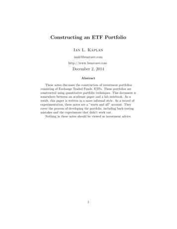
The table below shows the numeric portfolio weights. Portfolio weights arerounded to two decimal 4XOP0.00Table 8: Portfolio 65XSD5.61Table 9: Column Sum of WeightsFigure 4 shows the cumulative gain for the portfolio, along with the S&P 500benchmark. This is the ĜSPC index, not the S&P 500 ETF (SPY). Bychoosing the index rather than a tradable asset there is a consistentbenchmark.15
1.00.8Value1.21.4Quarterly Long Only Portfolio and S&P 5000.6PortfolioS&P 500Aug 08Apr 09Dec 09Sep 10May 11Jan 12Oct 12Jun 13Feb 14Oct 14DateFigure 4: Portfolio Cumulative Return with SP 500 ReturnThe draw-down chart is shown below in Figure 516
0.2 0.3Drawdown 0.10.0Portfolio and S&P 500 Drawdown 0.4PortfolioS&P 500Aug 08Apr 09Dec 09Sep 10May 11Jan 12Oct 12Jun 13Feb 14Oct 14DateFigure 5: Portfolio and SP 500 DrawdownThe information ratio is:IR E[Rp Rb ]αE[Rp Rb ] p σωvar(Rp Rb )(1)Using the S&P 500 as the benchmark, the information ratio of this portfoliois 0.0016884.As Figure 4 shows, this portfolio has performance that is very similar to thebenchmark.For taxable funds, the S&P 500 would be a better choice than this portfolio,which is traded every quarter.A holding period of less than a year-and-a-day will incur short term capitalgains taxes. Short-term capital gains are taxed at the income tax rate (e.g.,if your tax rate is 28 percent, the short-term capital gains tax will be 28percent).17
In contrast, long-term capital gains (for stocks held at least a year and a day)are 15 percent. The higher short-term capital gains rate incurs a 13 percentpenalty compared to simply holding the S&P 500 ETF (SPY).If a portfolio has performance that is similar to the benchmark (as is thecase here), the tax consequences of short term capital gains mean that itwould be better to purchase the benchmark and hold it for at least a year.Mean-Variance and Equally Weighted PortfoliosIn this section, for the universe of 10 ETFs (Table 1), an equally equallyweighted portfolio is compared to a Markowitz style mean-variance portfolio.The previous portfolio, shown in Figure 4, is not a classic mean varianceportfolio. This portfolio uses the functions shown in Table 7 to estimate thefuture return. This future return estimate is then used in portfoliooptimization.A Markowitz style mean-variance portfolio uses the mean to estimate thefuture return. The mean tends to be negatively correlated with the futurereturn, but mean-variance portfolio models do not attempt to correct for this.As Table 5 shows, the mean is not strongly correlated with future returns.The difference in the estimation of the future return accounts for thedifference between the portfolio shown in Figure 4 and the mean-varianceportfolio shown in the plot below.18
1.8MV, EQ and S&P 500 Portfolios1.20.60.81.0Value1.41.6Mean VarianceEqual WeightS&P 500Aug 08Apr 09Dec 09Sep 10May 11Jan 12Oct 12Jun 13Feb 14Oct 14DateFigure 6: MV Portfolio, Eq. Weighted and SP 500As Figure 6 shows, the equally weighted portfolio performs better than themean-variance portfolio and the portfolio in 4. The equally weightedportfolio also has low turnover (resulting in a lower tax rate). If the taxpenalty is taken into account, the equally weighted portfolio may be one ofthe top performing portfolios described in this paper.Predicting Returns, ReduxIn calculating the forecasted return for the first portfolio, an adjustmentfactor is used to adjust for negative correlation (in the case of XHB andXPH). The correlation adjustment and the choice of mean function (mean,EMA or OLS) is based on future information (e.g., over-fitting)19
Segmented Linear ModelThe more accurately the future return can be estimated, the more likely it isthat the portfolio will realize its target return. This section investigatesusing a segmented linear model to predict future returns. The motivation forthis was the idea that a segmented linear model would produce an moreaccurate estimate of the local mean.A segmented linear model maps a set of least squares lines through a timeseries. These fitted lines are the mean through the local distributions.A segmented linear model is created using the close price. An example isshown below in Figure 7. The return can be calculated from the segmentedlinear model result.30313233Close PriceLinear Model29XHB Weekly Close Price34As with the models discussed previously, one year (52 weeks) of past data isused to develop a prediction of the return, one quarter ahead.NovJanMarMayJulSepDate 2013 2014Figure 7: XHB Segmented Linear Model and Close Price20Nov
A return sequence is calculated from the fitted values from the linear model.The predicted return is the mean of the fitted values. By using the fittedvalues from the linear model, there is, in theory, less noise and the pricetrend is captured.The table below compares the mean, the segmented linear model mean andthe EMA on the segmented linear model 23LM 0.0036-0.01300.0014-0.0018-0.0299The tables below shows the correlation between the values predicted by themean, EMA and segmented linear model functions with the actual futurereturn.Mean functions vs. 2-week ahead ean functions vs. 4-week ahead 0.19020.0960-0.3072Mean functions vs. 8-week ahead 20.0914XLU0.02860.02970.0475Mean functions vs. 12-week ahead 80.0049XLU0.15180.25860.049321
As the comparison point moves out in time (from 2 to 12 weeks), thecorrelations increase. The EMA is a notably better predictor in most casesthan the segmented linear model, the mean or ordinary least squares.Looking Back at the Hand Selected PortfolioThe portfolio chosen from the hand selected ETFs by the optimizer for theMay to August 2014 time period was:1HYGXLU20.240.76The optimization was not constrained to limit portfolio weight and therewere only nine ETFs in the ETF universe.This portfolio may suffers from over-fitting. In selecting the return forecastfunctions and the correlation adjustment, future knowledge is used to selectthe function with the bast historical correlation and to select the adjustmentfactor (to adjust for negative correlation). Small changes in the meanfunctions and the correlation adjustment result in large changes on theportfolio result. This suggests that these factors are not stable.Another problem is that the correlation adjustments for the various functionsare estimated from the distributions of only a few assets.Portfolio ReduxThe rest of the paper investigates portfolios that have better performancethan the portfolio shown in Figure 4, which was constructed from the handselected set of ETFs.Asset SelectionPortfolio returns are extremely sensitive to the choice of assets. Quantitativetechniques cannot turn lead into gold. A portfolio algorithm can onlyproduce returns within its universe of assets. For example, the maximum22
gain-loss and maximum Sharpe ratio algorithm produced extremely poorreturns with an initial set of ETFs. Much better returns were produced withthe etf.com list, discussed below.The literature on asset selection for stocks goes back at least as far as thefirst edition of Graham and Dodd’s 1934 book Securities Analysis. A varietyof factors have been proposed for selecting the stocks for a portfolio.ETFs are collections of stocks and other assets (like futures contracts) thatcan be traded without tax consequences. This makes the analysis of ETFsmore complicated than single stocks. ETFs also have a wide variety of assetsand strategies. Their complex nature makes ETFs more difficult to select onan empirical basis.The portfolios select ETFs on the basis of past performance. The problemwith always looking at the past, without any tools to forecast futureperformance, is that sometimes the desired performance is also in the past.Selecting ETFsIn the case of stocks, the universe can be selected from the stocks that makeup an index, like the S&P 500. With ETFs there is no canonical choice forthe ETF universe.Originally a list of ETFs was constructed from a list from the Morningstarweb site. The Morningstar ETF filter is difficult to use and does not allowdata to be exported to a CSV file. Morningstar has also placed a number offeatures behind a pay wall.I later discovered that a better source of ETF information is the etf.com website. This site allows ETFs to be selected on the basis of minimumcapitalization (among other criteria). The data can be easily exported inCSV format.The ”settings” used in the etf.com screen are: Efficiency: 80 and above AUM: 10 million 3 Mo Return: 0 percent23
1 Year Re
Unlike index mutual funds, ETFs trade like stocks. A portfolio constructed from a few ETFs have some level of diversi cation, since an ETF itself is composed on a portfolio of assets. ETFs also have tax advantages compared to mutual funds or index funds (unlike mutual funds, trading within an ETF does not incur tax liability). Past is Prologue