Transcription
Chapter 3Basic MapReduce AlgorithmDesignThis is a post-production manuscript of: Jimmy Lin and Chris Dyer. Data-IntensiveText Processing with MapReduce. Morgan & Claypool Publishers, 2010. This version was compiled on December 25, 2017.A large part of the power of MapReduce comes from its simplicity: in additionto preparing the input data, the programmer needs only to implement the mapper, the reducer, and optionally, the combiner and the partitioner. All otheraspects of execution are handled transparently by the execution framework—on clusters ranging from a single node to a few thousand nodes, over datasetsranging from gigabytes to petabytes. However, this also means that any conceivable algorithm that a programmer wishes to develop must be expressedin terms of a small number of rigidly-defined components that must fit together in very specific ways. It may not appear obvious how a multitude ofalgorithms can be recast into this programming model. The purpose of thischapter is to provide, primarily through examples, a guide to MapReduce algorithm design. These examples illustrate what can be thought of as “designpatterns” for MapReduce, which instantiate arrangements of components andspecific techniques designed to handle frequently-encountered situations acrossa variety of problem domains. Two of these design patterns are used in thescalable inverted indexing algorithm we’ll present later in Chapter 4; conceptspresented here will show up again in Chapter 5 (graph processing) and Chapter 7 (expectation-maximization algorithms).Synchronization is perhaps the most tricky aspect of designing MapReducealgorithms (or for that matter, parallel and distributed algorithms in general).Other than embarrassingly-parallel problems, processes running on separatenodes in a cluster must, at some point in time, come together—for example,to distribute partial results from nodes that produced them to the nodes thatwill consume them. Within a single MapReduce job, there is only one opportunity for cluster-wide synchronization—during the shuffle and sort stage where
intermediate key-value pairs are copied from the mappers to the reducers andgrouped by key. Beyond that, mappers and reducers run in isolation withoutany mechanisms for direct communication. Furthermore, the programmer haslittle control over many aspects of execution, for example: Where a mapper or reducer runs (i.e., on which node in the cluster). When a mapper or reducer begins or finishes. Which input key-value pairs are processed by a specific mapper. Which intermediate key-value pairs are processed by a specific reducer.Nevertheless, the programmer does have a number of techniques for controllingexecution and managing the flow of data in MapReduce. In summary, they are:1. The ability to construct complex data structures as keys and values tostore and communicate partial results.2. The ability to execute user-specified initialization code at the beginning ofa map or reduce task, and the ability to execute user-specified terminationcode at the end of a map or reduce task.3. The ability to preserve state in both mappers and reducers across multipleinput or intermediate keys.4. The ability to control the sort order of intermediate keys, and thereforethe order in which a reducer will encounter particular keys.5. The ability to control the partitioning of the key space, and therefore theset of keys that will be encountered by a particular reducer.It is important to realize that many algorithms cannot be easily expressed asa single MapReduce job. One must often decompose complex algorithms intoa sequence of jobs, which requires orchestrating data so that the output of onejob becomes the input to the next. Many algorithms are iterative in nature, requiring repeated execution until some convergence criteria—graph algorithmsin Chapter 5 and expectation-maximization algorithms in Chapter 7 behavein exactly this way. Often, the convergence check itself cannot be easily expressed in MapReduce. The standard solution is an external (non-MapReduce)program that serves as a “driver” to coordinate MapReduce iterations.This chapter explains how various techniques to control code execution anddata flow can be applied to design algorithms in MapReduce. The focus is bothon scalability—ensuring that there are no inherent bottlenecks as algorithmsare applied to increasingly larger datasets—and efficiency—ensuring that algorithms do not needlessly consume resources and thereby reducing the cost ofparallelization. The gold standard, of course, is linear scalability: an algorithmrunning on twice the amount of data should take only twice as long. Similarly,
an algorithm running on twice the number of nodes should only take half aslong.The chapter is organized as follows: Section 3.1 introduces the important concept of local aggregation in MapReduce and strategies for designing efficient algorithms that minimize theamount of partial results that need to be copied across the network. Theproper use of combiners is discussed in detail, as well as the “in-mappercombining” design pattern. Section 3.2 uses the example of building word co-occurrence matrices onlarge text corpora to illustrate two common design patterns, which wedub “pairs” and “stripes”. These two approaches are useful in a largeclass of problems that require keeping track of joint events across a largenumber of observations. Section 3.3 shows how co-occurrence counts can be converted into relativefrequencies using a pattern known as “order inversion”. The sequencingof computations in the reducer can be recast as a sorting problem, wherepieces of intermediate data are sorted into exactly the order that is required to carry out a series of computations. Often, a reducer needs tocompute an aggregate statistic on a set of elements before individual elements can be processed. Normally, this would require two passes overthe data, but with the “order inversion” design pattern, the aggregatestatistic can be computed in the reducer before the individual elementsare encountered. This may seem counter-intuitive: how can we computean aggregate statistic on a set of elements before encountering elements ofthat set? As it turns out, clever sorting of special key-value pairs enablesexactly this. Section 3.4 provides a general solution to secondary sorting, which is theproblem of sorting values associated with a key in the reduce phase. Wecall this technique “value-to-key conversion”.3.1Local AggregationIn the context of data-intensive distributed processing, the single most important aspect of synchronization is the exchange of intermediate results, from theprocesses that produced them to the processes that will ultimately consumethem. In a cluster environment, with the exception of embarrassingly-parallelproblems, this necessarily involves transferring data over the network. Furthermore, in Hadoop, intermediate results are written to local disk before beingsent over the network. Since network and disk latencies are relatively expensive compared to other operations, reductions in the amount of intermediatedata translate into increases in algorithmic efficiency. In MapReduce, localaggregation of intermediate results is one of the keys to efficient algorithms.Through use of the combiner and by taking advantage of the ability to preserve
Algorithm 3.1 Word count (repeated from Algorithm 2.1)The mapper emits an intermediate key-value pair for each word in an inputdocument. The reducer sums up all counts for each word.123456class Mapper {def map(key: Long, value: Text) {for (word - tokenize(value)) {emit(word, 1)}}789101112131415class Reducer {def reduce(key: Text, values: Iterable[Int]) {for (value - values) {sum value}emit(key, sum)}}state across multiple inputs, it is often possible to substantially reduce both thenumber and size of key-value pairs that need to be shuffled from the mappersto the reducers.Combiners and In-Mapper CombiningWe illustrate various techniques for local aggregation using the simple wordcount example presented in Section 2.2. For convenience, Algorithm 3.1 repeatsthe pseudo-code of the basic algorithm, which is quite simple: the mapper emitsan intermediate key-value pair for each term observed, with the term itself asthe key and a value of one; reducers sum up the partial counts to arrive at thefinal count.The first technique for local aggregation is the combiner, already discussedin Section 2.4. Combiners provide a general mechanism within the MapReduce framework to reduce the amount of intermediate data generated bythe mappers—recall that they can be understood as “mini-reducers” that process the output of mappers. In this example, the combiners aggregate termcounts across the documents processed by each map task. This results in a reduction in the number of intermediate key-value pairs that need to be shuffledacross the network—from the order of total number of terms in the collectionto the order of the number of unique terms in the collection.11 More precisely, if the combiners take advantage of all opportunities for local aggregation,the algorithm would generate at most m V intermediate key-value pairs, where m is thenumber of mappers and V is the vocabulary size (number of unique terms in the collection),since every term could have been observed in every mapper. However, there are two additionalfactors to consider. Due to the Zipfian nature of term distributions, most terms will not beobserved by most mappers (for example, terms that occur only once will by definition only be
Algorithm 3.2 Word count mapper using associative arraysThe mapper builds a histogram of all words in each input document beforeemitting key-value pairs for unique words observed.1234567891011class Mapper {def map(key: Long, value: Text) {val counts new Map()for (word - tokenize(value)) {counts(word) 1}for ((k, v) - counts) {emit(k, v)}}}An improvement on the basic algorithm is shown in Algorithm 3.2 (themapper is modified but the reducer remains the same as in Algorithm 3.1 andtherefore is not repeated). An associative array (i.e., Map in Java) is introducedinside the mapper to tally up term counts within a single document: instead ofemitting a key-value pair for each term in the document, this version emits akey-value pair for each unique term in the document. Given that some wordsappear frequently within a document (for example, a document about dogs islikely to have many occurrences of the word “dog”), this can yield substantialsavings in the number of intermediate key-value pairs emitted, especially forlong documents.This basic idea can be taken one step further, as illustrated in the variantof the word count algorithm in Algorithm 3.3 (once again, only the mapper ismodified). The workings of this algorithm critically depends on the details ofhow map and reduce tasks in Hadoop are executed, discussed in Section 2.6.Recall, a (Java) mapper object is created for each map task, which is responsiblefor processing a block of input key-value pairs. Prior to processing any inputkey-value pairs, the mapper’s setup method is called, which is an API hook foruser-specified code. In this case, we initialize an associative array for holdingterm counts. Since it is possible to preserve state across multiple calls of themap method (for each input key-value pair), we can continue to accumulatepartial term counts in the associative array across multiple documents, andemit key-value pairs only when the mapper has processed all documents. Thatis, emission of intermediate data is deferred until the cleanup method in thepseudo-code. Recall that this API hook provides an opportunity to executeuser-specified code after the map method has been applied to all input keyvalue pairs of the input data split to which the map task was assigned.With this technique, we are in essence incorporating combiner functionalityobserved by one mapper). On the other hand, combiners in Hadoop are treated as optionaloptimizations, so there is no guarantee that the execution framework will take advantage ofall opportunities for partial aggregation.
Algorithm 3.3 Word count mapper using the“in-mapper combining”The mapper builds a histogram of all input documents processed before emitting key-value pairs for unique words observed.12class Mapper {val counts new Map()3def map(key: Long, value: Text) {for (word - tokenize(value)) {counts(word) 1}}456789def cleanup() {for ((k, v) - counts) {emit(k, v)}}101112131415}directly inside the mapper. There is no need to run a separate combiner,since all opportunities for local aggregation are already exploited.2 This isa sufficiently common design pattern in MapReduce that it’s worth giving ita name, “in-mapper combining”, so that we can refer to the pattern moreconveniently throughout the book. We’ll see later on how this pattern can beapplied to a variety of problems. There are two main advantages to using thisdesign pattern:First, it provides control over when local aggregation occurs and how itexactly takes place. In contrast, the semantics of the combiner is underspecifiedin MapReduce. For example, Hadoop makes no guarantees on how many timesthe combiner is applied, or that it is even applied at all. The combiner isprovided as a semantics-preserving optimization to the execution framework,which has the option of using it, perhaps multiple times, or not at all (or evenin the reduce phase). In some cases (although not in this particular example),such indeterminism is unacceptable, which is exactly why programmers oftenchoose to perform their own local aggregation in the mappers.Second, in-mapper combining will typically be more efficient than usingactual combiners. One reason for this is the additional overhead associatedwith actually materializing the key-value pairs. Combiners reduce the amountof intermediate data that is shuffled across the network, but don’t actuallyreduce the number of key-value pairs that are emitted by the mappers in thefirst place. With the algorithm in Algorithm 3.2, intermediate key-value pairsare still generated on a per-document basis, only to be “compacted” by the2 Leaving aside the minor complication that in Hadoop, combiners can be run in thereduce phase also (when merging intermediate key-value pairs from different map tasks).However, in practice it makes almost no difference either way.
combiners. This process involves unnecessary object creation and destruction(garbage collection takes time), and furthermore, object serialization and deserialization (when intermediate key-value pairs fill the in-memory buffer holdingmap outputs and need to be temporarily spilled to disk). In contrast, with inmapper combining, the mappers will generate only those key-value pairs thatneed to be shuffled across the network to the reducers.There are, however, drawbacks to the in-mapper combining pattern. First,it breaks the functional programming underpinnings of MapReduce, since stateis being preserved across multiple input key-value pairs. Ultimately, this isn’ta big deal, since pragmatic concerns for efficiency often trump theoretical “purity”, but there are practical consequences as well. Preserving state acrossmultiple input instances means that algorithmic behavior may depend on theorder in which input key-value pairs are encountered. This creates the potential for ordering-dependent bugs, which are difficult to debug on large datasetsin the general case (although the correctness of in-mapper combining for wordcount is easy to demonstrate). Second, there is a fundamental scalability bottleneck associated with the in-mapper combining pattern. It critically dependson having sufficient memory to store intermediate results until the mapper hascompletely processed all key-value pairs in an input split. In the word countexample, the memory footprint is bound by the vocabulary size, since it istheoretically possible that a mapper encounters every term in the collection.Heap’s Law, a well-known result in information retrieval, accurately models thegrowth of vocabulary size as a function of the collection size—the somewhatsurprising fact is that the vocabulary size never stops growing.3 Therefore, thealgorithm in Algorithm 3.3 will scale only up to a point, beyond which theassociative array holding the partial term counts will no longer fit in memory.4One common solution to limiting memory usage when using the in-mappercombining technique is to “block” input key-value pairs and “flush” in-memorydata structures periodically. The idea is simple: instead of emitting intermediate data only after every key-value pair has been processed, emit partial resultsafter processing every n key-value pairs. This is straightforwardly implementedwith a counter variable that keeps track of the number of input key-value pairsthat have been processed. As an alternative, the mapper could keep track ofits own memory footprint and flush intermediate key-value pairs once memoryusage has crossed a certain threshold. In both approaches, either the blocksize or the memory usage threshold needs to be determined empirically: withtoo large a value, the mapper may run out of memory, but with too small avalue, opportunities for local aggregation may be lost. Furthermore, in Hadoop3 In more detail, Heap’s Law relates the vocabulary size V to the collection size as follows:V kT b , where T is the number of tokens in the collection. Typical values of the parametersk and b are: 30 k 100 and b 0.5 ([101], p. 81).4 A few more details: note what matters is that the partial term counts encountered withinparticular input split fits into memory. However, as collection sizes increase, one will oftenwant to increase the input split size to limit the growth of the number of map tasks (in orderto reduce the number of distinct copy operations necessary to shuffle intermediate data overthe network).
physical memory is split between multiple tasks that may be running on a nodeconcurrently; these tasks are all competing for finite resources, but since thetasks are not aware of each other, it is difficult to coordinate resource consumption effectively. In practice, however, one often encounters diminishing returnsin performance gains with increasing buffer sizes, such that it is not worth theeffort to search for an optimal buffer size (personal communication, Jeff Dean).In MapReduce algorithms, the extent to which efficiency can be increasedthrough local aggregation depends on the size of the intermediate key space,the distribution of keys themselves, and the number of key-value pairs thatare emitted by each individual map task. Opportunities for aggregation, afterall, come from having multiple values associated with the same key (whetherone uses combiners or employs the in-mapper combining pattern). In the wordcount example, local aggregation is effective because many words are encountered multiple times within a map task. Local aggregation is also an effectivetechnique for dealing with reduce stragglers (see Section 2.3) that result froma highly-skewed (e.g., Zipfian) distribution of values associated with intermediate keys. In our word count example, we do not filter frequently-occurringwords: therefore, without local aggregation, the reducer that’s responsible forcomputing the count of ‘the’ will have a lot more work to do than the typicalreducer, and therefore will likely be a straggler. With local aggregation (eithercombiners or in-mapper combining), we substantially reduce the number ofvalues associated with frequently-occurring terms, which alleviates the reducestraggler problem.Algorithmic Correctness with Local AggregationAlthough use of combiners can yield dramatic reductions in algorithm runningtime, care must be taken in applying them. Since combiners in Hadoop areviewed as optional optimizations, the correctness of the algorithm cannot depend on computations performed by the combiner or depend on them evenbeing run at all. In any MapReduce program, the reducer input key-value typemust match the mapper output key-value type: this implies that the combinerinput and output key-value types must match the mapper output key-valuetype (which is the same as the reducer input key-value type). In cases wherethe reduce computation is both commutative and associative, the reducer canalso be used (unmodified) as the combiner (as is the case with the word countexample). In the general case, however, combiners and reducers are not interchangeable.Consider a simple example: we have a large dataset where input keys arestrings and input values are integers, and we wish to compute the mean ofall integers associated with the same key (rounded to the nearest integer). Areal-world example might be a large user log from a popular website, wherekeys represent user ids and values represent some measure of activity such aselapsed time for a particular session—the task would correspond to computingthe mean session length on a per-user basis, which would be useful for understanding user demographics. Algorithm 3.4 shows the pseudo-code of a simple
Algorithm 3.4 Compute the mean of values associated with the same keyThe mapper is the identify function; the mean is computed in the reducer.12345class Mapper {def map(key: Text, value: Int) {emit(key, value)}}6789101112131415class Reducer {def reduce(key: Text, values: Iterable[Int]) {for (value - values) {sum valuecnt 1}emit(key, sum/cnt)}}algorithm for accomplishing this task that does not involve combiners. Weuse an identity mapper, which simply passes all input key-value pairs to thereducers (appropriately grouped and sorted). The reducer keeps track of therunning sum and the number of integers encountered. This information is usedto compute the mean once all values are processed. The mean is then emittedas the output value in the reducer (with the input string as the key).This algorithm will indeed work, but suffers from the same drawbacks as thebasic word count algorithm in Algorithm 3.1: it requires shuffling all key-valuepairs from mappers to reducers across the network, which is highly inefficient.Unlike in the word count example, the reducer cannot be used as a combiner inthis case. Consider what would happen if we did: the combiner would computethe mean of an arbitrary subset of values associated with the same key, andthe reducer would compute the mean of those values. As a concrete example,we know that:Mean(1, 2, 3, 4, 5) 6 Mean(Mean(1, 2), Mean(3, 4, 5))(3.1)In general, the mean of means of arbitrary subsets of a set of numbers is notthe same as the mean of the set of numbers. Therefore, this approach wouldnot produce the correct result.5So how might we properly take advantage of combiners? An attempt isshown in Algorithm 3.5. The mapper remains the same, but we have added acombiner that partially aggregates results by computing the numeric components necessary to arrive at the mean. The combiner receives each string and5 There is, however, one special case in which using reducers as combiners would producethe correct result: if each combiner computed the mean of equal-size subsets of the values.However, since such fine-grained control over the combiners is impossible in MapReduce,such a scenario is highly unlikely.
Algorithm 3.5 Compute the mean of values associated with the same keyNote that this algorithm is incorrect. The mismatch between combiner inputand output key-value types violates the MapReduce programming model.1234class Mapper {def map(key: Text, value: Int) emit(key, value)}567891011121314class Combiner {def reduce(key: Text, values: Iterable[Int]) {for (value - values) {sum valuecnt 1}emit(key, (sum, cnt))}}15161718192021222324class Reducer {def reduce(key: Text, values: Iterable[Pair]) {for ((s, c) - values) {sum scnt c}emit(key, sum/cnt)}}the associated list of integer values, from which it computes the sum of thosevalues and the number of integers encountered (i.e., the count). The sum andcount are packaged into a pair, and emitted as the output of the combiner, withthe same string as the key. In the reducer, pairs of partial sums and countscan be aggregated to arrive at the mean. Up until now, all keys and valuesin our algorithms have been primitives (string, integers, etc.). However, thereare no prohibitions in MapReduce for more complex types,6 and, in fact, thisrepresents a key technique in MapReduce algorithm design that we introducedat the beginning of this chapter. We will frequently encounter complex keysand values throughput the rest of this book.Unfortunately, this algorithm will not work. Recall that combiners musthave the same input and output key-value type, which also must be the sameas the mapper output type and the reducer input type. This is clearly notthe case. To understand why this restriction is necessary in the programmingmodel, remember that combiners are optimizations that cannot change thecorrectness of the algorithm. So let us remove the combiner and see what6 In Hadoop, either custom types or types defined using a library such as Protocol Buffers,Thrift, or Avro.
Algorithm 3.6 Compute the mean of values associated with the same keyThis algorithm correctly takes advantage of combiners by storing the sum andcount separately as a pair.1234class Mapper {def map(key: Text, value: Int) emit(key, (value, 1))}567891011121314class Combiner {def reduce(key: Text, values: Iterable[Pair]) {for ((s, c) - values) {sum scnt c}emit(key, (sum, cnt))}}15161718192021222324class Reducer {def reduce(key: Text, values: Iterable[Pair]) {for ((s, c) - values) {sum scnt c}emit(key, sum/cnt)}}happens: the output value type of the mapper is integer, so the reducer expectsto receive a list of integers as values. But the reducer actually expects a list ofpairs! The correctness of the algorithm is contingent on the combiner runningon the output of the mappers, and more specifically, that the combiner isrun exactly once. Recall from our previous discussion that Hadoop makes noguarantees on how many times combiners are called; it could be zero, one, ormultiple times. This violates the MapReduce programming model.Another stab at the solution is shown in Algorithm 3.6, and this time, thealgorithm is correct. In the mapper we emit as the value a pair consistingof the integer and one—this corresponds to a partial count over one instance.The combiner separately aggregates the partial sums and the partial counts(as before), and emits pairs with updated sums and counts. The reducer issimilar to the combiner, except that the mean is computed at the end. Inessence, this algorithm transforms a non-associative operation (mean of numbers) into an associative operation (element-wise sum of a pair of numbers,with an additional division at the very end).Let us verify the correctness of this algorithm by repeating the previousexercise: What would happen if no combiners were run? With no combiners,
Algorithm 3.7 Compute the mean of values associated with the same keyThis mapper illustrates the in-mapper combining design pattern. The reduceris the same as in Algorithm 3.6123class Mapper {val sums new Map()val counts new Map()4def map(key: Text, value: Int) {sums(key) valuecounts(key) 1}56789def cleanup() {for (key - counts.keys) {emit(key, (sums(key), counts(key)))}}101112131415}the mappers would send pairs (as values) directly to the reducers. There wouldbe as many intermediate pairs as there were input key-value pairs, and eachof those would consist of an integer and one. The reducer would still arrive atthe correct sum and count, and hence the mean would be correct. Now addin the combiners: the algorithm would remain correct, no matter how manytimes they run, since the combiners merely aggregate partial sums and countsto pass along to the reducers. Note that although the output key-value typeof the combiner must be the same as the input key-value type of the reducer,the reducer can emit final key-value pairs of a different type.Finally, in Algorithm 3.7, we present an even more efficient algorithm thatexploits the in-mapper combining pattern. Inside the mapper, the partial sumsand counts associated with each string are held in memory across input keyvalue pairs. Intermediate key-value pairs are emitted only after the entire inputsplit has been processed; similar to before, the value is a pair consisting of thesum and count. The reducer is exactly the same as in Algorithm 3.6. Movingpartial aggregation from the combiner directly into the mapper is subjected toall the tradeoffs and caveats discussed earlier this section, but in this case thememory footprint of the data structures for holding intermediate data is likelyto be modest, making this variant algorithm an attractive option.3.2Pairs and StripesOne common approach for synchronization in MapReduce is to construct complex keys and values in such a way that data necessary for a computation arenaturally brought together by the execution framework. We first touched onthis technique in the previous section, in the context of “packaging” partial
sums and counts in a complex value (i.e., pair) that is passed from mapperto combiner to reducer. Building on previously published work [54, 94], thissection introduces two common design patterns we have dubbed “pairs” and“stripes” that exemplify this strategy.As a running example, we focus on the problem of building word cooccurrence matrices from large corpora, a common task in corpus linguisticsand statistical natural language processing. Formally, the co-occurrence matrix of a corpus is a square n n matrix where n is the number of uniquewords in the corpus (i.e., the vocabulary size). A cell mij contains the numberof times word wi co-occurs with word wj within a specific context—a naturalunit such as a sentence, paragraph, or a document, or a certain window of mwords (where m is an applic
Basic MapReduce Algorithm Design This is a post-production manuscript of: Jimmy Lin and Chris Dyer. Data-Intensive Text Processing with MapReduce. Morgan & Claypool Publishers, 2010. This ver-sion was compiled on December 25, 2017. A large part of the power of MapReduce comes from its simplicity: in addition