WIXLIB

FFT, total energy, and energy spectral density computations in MATLABAaron ScherEverything presented here is specifically focused on non-periodic signals with finite energy (alsocalled “energy signals”).Part 1. THEORYInstantaneous power of continuous-time signals:Let 𝑥 𝑡 be a real (i.e. no imaginary part) signal. If 𝑥 𝑡 represents voltage across a 1 W resistor,then the instantaneous power dissipated by Ohmic losses in the resistor is:𝑝 𝑡 % & '( 𝑥 𝑡 ).(Instantaneous power in [W] [J/s])(1)Total energy of continuous-time signals:The total energy dissipated across the resistor is the time-integral of the instantaneous power:.𝑝/.𝐸, 𝑡 𝑑𝑡 .𝑥/.𝑡 ) 𝑑𝑡.(Total signal energy in [J])(2)A signal with a finite energy 𝐸, (i.e. 𝐸, ) is called an “energy signal”. We are focusing solelyon energy signals here.Continuous time Fourier transform (CTFT) pair:Recall the CTFT:𝑋 𝑓 .𝑥/.𝑡 𝑒 /5)67& 𝑑𝑡(3)Energy of continuous-time signals computed in frequency domainIt can be shown using Parseval’s theorem that the total energy can also be computed in thefrequency domain:𝐸, ./.𝑋 𝑓)𝑑𝑓.(Total signal energy in [J] computed in frequency domain)(4)Compare equation (4) with (2). These are two ways equations to compute the total energy E.Energy spectral densityLooking at Equation (5), we see that we can define an energy spectral density (ESD) given by:Ψ, 𝑓 𝑋 𝑓 ) .(Energy spectral density in [J/Hz])(5)1

Part 2. MATLABOur goal in this section is to use MATLAB to plot the amplitude spectrum, energy spectraldensity, and numerically estimate the total energy Eg.First, let’s sample!How do we sample a signal 𝑥 𝑡 in MATLAB? For ease, let’s work specifically on an example(you can easily generalize what is presented here to other signals). Suppose our signal is a small“piece” of sinusoid with frequency 𝑓; described by the function:0.𝑥 𝑡 sin 2𝜋𝑓; 𝑡 ,0,𝑡 1 1 𝑡 1𝑡 1(6)where the units for time are in seconds. Given 𝑓; we need to choose a sampling frequency 𝑓Gthat is sufficiently high (should be higher than Nyquist rate to avoid aliasing ). For this example,let us choose 𝑓; 2 𝐻𝑧 and a sampling frequency 𝑓G 20 𝐻𝑧. The MATLAB code looks likethis:1234567-f0 2; %center frequency [Hz]fs 20; %sample rate [Hz]Ts 1/fs; %sample period [s]Tbegin -1; %Our signal is nonzero over the time interval [Tbegin Tend].Tend 1;t [Tbegin:Ts:Tend]; %define array with sampling timesx sin(2*pi*f0*t); %define discrete-time function. This is x[n].Mathematically, our discrete-time function x[n] (defined in line 7 of code above) is equal to thecontinuous-function 𝑥 𝑡 (ignoring quantization error) at discrete points in time. Hence, wemay write:(7)𝑥[𝑛] 𝑥 𝑡Mwhere 𝑡M are the sampling times defined in line 6 of code above:𝑡M 𝑇OPQRS 𝑛 1 𝑇G ,𝑛 1 𝑁;(8)where 𝑇G 1 𝑓G is the sampling period, 𝑁; is the final index of x[n], i.e. 𝑁; length(x), and𝑇OPQRS is the initial time where the finite-energy signal x(t) is nonzero (e.g. for the signal given byequation (6), 𝑇OPQRS 1 seconds). In MATLAB, the indices n always start at 1 and are positive.This can cause confusion, since in other programming languages indices commonly start at 0.So, in MATLAB, x[0] would give an error. You must start with an index of 1; x[1] would be fine.2

If we are interested in evaluating 𝑥 𝑡M at some specific time, say at t 0, we can figure out theindex n that corresponds to t 0, and plug it in to our expression for x. However, the easier wayis to simply plot our function x and look at the value of this function at t 0, as done below.8 - figure(1)9 - plot(t,x)10 - grid on11 - xlabel('Time (seconds)','fontsize',14)12 - .60.81Time (seconds)Figure 1. Plot of 𝑥 𝑛 𝑥 𝑡M . Discrete points are connected by straight lines and the x-axis islabeled as time in seconds. This gives the illusion that this is a plot of a true continuous timesignal 𝑥 𝑡 . It’s actually a plot of a discrete time signal.From the plot above, it is clear that the function x(t) 0 at t 0. If we weren’t in the mood toplot, we could also find the index value that corresponds to t 0, and plug that directly into x tofind the value of x at t 0, as shown in the code below:13 14 -index find(t 0,1) %find index n corresponding to t 0.This returns 21x(index) %This returns 0, as expected.Total energy approximationWe can numerically estimate the total energy by approximating equation (2) with a Riemannsum:Eg 𝑇G n 1𝑥[𝑛])(Estimate total signal energy in [J])(9)3

MATLAB’s FFT functionMatlab’s fft function is an efficient algorithm for computing the discrete Fourier transform(DFT) of a function. To find the double-sided spectrum you need to use the fftshiftfunction.Equation (3) shows how to manually compute the continuous time Fourier transform (CTFT)𝑋 𝑓 of a continuous time function 𝑥 𝑡 . Instead of using an integral, we can use MATLAB tonumerically compute the CFT at discrete frequency points 𝑓 as follows:𝑋 𝑓 a7bfftshift(fft(x,N))(10)where N is the number of frequency points in the FFT, and 𝑓 are discrete frequency points:𝑓 7b) 𝑛 17b /a,𝑛 1 𝑁(11)Recall that 𝑁; length(x) is the number of discrete time points of the original signal 𝑥[𝑛].In general 𝑁; 𝑁, and you are free to choose N as large as you want (so long as yourcomputer can handle it). In fact, you will generally set N N0. A good value for N is N 216.The code below demonstrates how to calculate and plot the -N 2 16; %good general value for FFT (this is the number of discretepoints in the FFT.)y fft(x,N); %compute FFT! There is a lot going on "behind the scenes"with this one line of code.z fftshift(y); %Move the zero-frequency component to the center of the%array. This is used for finding the double-sided spectrum (as opposedto the single-sided spectrum).f vec [0:1:N-1]*fs/N-fs/2; %Create frequency vector (this is an arrayof numbers. Each number corresponds to a discrete point in frequencyin which we shall evaluate and plot the function.)amplitude spectrum abs(z)/fs %Extract the amplitude of thespectrum. Here we also apply a scaling factor of 1/fs so thatthe amplitude of the FFT at a frequency component equals that of theCFT and to preserve Parseval’s theorem.figure(2)plot(f vec,amplitude spectrum);set(gca,'FontSize',18) %set font size of axis tick labels to 18xlabel('Frequency 18)title('Amplitude spectra','fontsize',18)grid onset(gcf,'color','w');%set background color from grey(default) to whiteaxis tight4

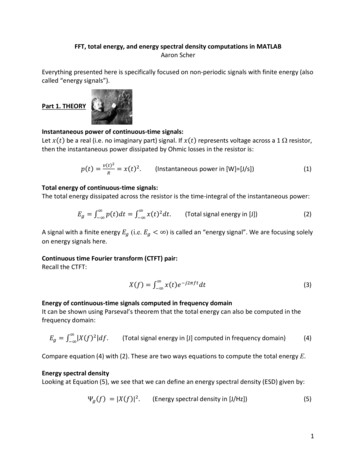
Amplitude spectra1Amplitude0.80.60.40.20-10-50Frequency [Hz]5Figure 2Once you have computed 𝑋 𝑓 using equation (10), you can then numerically compute andplot the energy spectral density (ESD):Ψ, [𝑓 ] 𝑋 𝑓 ) .(Energy spectral density in [J/Hz])(12)The total energy can then be found by approximating equation (4) with a Riemann sum:Eg 7b n 1𝑋 𝑓 ).(Total signal energy in [J] computed in frequency domain)(13)The code below demonstrates how to calculate and plot the energy spectral density.-figure(3)plot(f vec,abs(amplitude spectrum). 2);xlabel('Frequency 18)title('Energy spectral density','fontsize',18)grid onset(gcf,'color','w'); %set background color to whiteaxis tightEnergy spectral 40.30.20.10-10-8-6-4-202468Frequency [Hz]Figure 35

We can now numerically calculate the total energy using either equation (9) or (13):%calculate total energy46 - Eg sum(x. 2)*Ts %using discrete time function x[n]47 - Eg sum(amplitude spectrum. 2)*fs/N %using ESDMATLAB returns Eg 1.000 for both methods. The units of energy are Joules [J].The full MATLAB code for the above example is pasted below. Simply save this code in an mfile and run the m-file.clc;clear all;f0 2; %center frequency [Hz]fs 20; %sample rate [Hz]Ts 1/fs; %sample period [s]Tbegin -1; %Our signal is nonzero over the time interval [Tbegin Tend]Tend 1;t [Tbegin:Ts:Tend]; %define array with discrete sampling times.x sin(2*pi*f0*t); %define discrete-time function. This is x[n].figure(1)plot(t,x)grid onxlabel('Time ize',14)N 2 16; %good general value for FFT (this is the number of discrete points in theFFT.)y fft(x,N); %compute FFT! There is a lot going on "behind the scenes" with%this one line of code.z fftshift(y); %Move the zero-frequency component to the center of the%array. This is used for finding the double-sided spectrum (as opposed to%the single-sided spectrum).f vec [0:1:N-1]*fs/N-fs/2; %Create frequency vector (this is an array of%numbers. Each number corresponds to a discrete point in frequency in which we%shall evaluate and plot the function.)amplitude spectrum abs(z)/fs; %Extract the amplitude of the spectrum%Here we also apply a scaling factor of 1/fs, so that the amplitude%of the FFT at a frequency component equals that of the the CFT and to%preserve Parseval's theorem.amplitude spectrum abs(z)*Ts;figure(2)plot(f vec,amplitude spectrum);set(gca,'FontSize',18) %set font size of axis tick labels to 18xlabel('Frequency 18)title('Amplitude spectra','fontsize',18)grid onset(gcf,'color','w'); %set background color from grey (default) to whiteaxis tightfigure(3)plot(f vec,abs(amplitude spectrum). 2);xlabel('Frequency 18)title('Energy spectral density','fontsize',18)grid onset(gcf,'color','w'); %set background color from grey (default) to whiteaxis tight%calculate total energyEg sum(x. 2)*Ts %using discrete time function x[n]Eg sum(amplitude spectrum. 2)*fs/N %Using ESD6

Part 3. One last thing – Autocorrelation MethodBelieve it or not, there is a second way to calculate the energy spectral density (ESD), Ψ, 𝑡 .Equation (5) presents one method for calculating Ψ, . But folks, in life we have choices. Let’sexamine the second method.First, the time autocorrelation function is defined as:𝜓, 𝜏 .𝑥/.𝑡 𝑥 𝑡 𝜏 𝑑𝑡.(Autocorrelation function)(14)It can be proved that the Fourier transform of the autocorrelation function is equal to the ESD,Ψ, 𝑡 , i.e.ℱ 𝜓, 𝜏 Ψ, 𝑓 𝑋 𝑓 )(FT of autocorrelation function is ESD)(15)In MATLAB, we can numerically compute the autocorrelation function presented in equation(14) using the xcorr function :𝜓, 𝜏M a7bxcorr(x,x)(16)We can then find the ESD by taking the FFT of 𝜓, 𝜏M . The MATAB code below shows how tocompute ESD using the autocorrelation method. Figure 4 shows a spectral plot of the ESD.Compare Figure 4 with Figure 3 – they are identical – which demonstrates the two differentmethods for yield identical results for the ESD.%This code continues from the previous code (i.e., x, Ts, fs, f vec and%N are already defined)%Below I demonstrate an alternative method to plot EST. This method%uses autocorrelationcor Ts*xcorr(x,x); %numerically compute autocorrelation.%cor Ts*conv(flipud(x),x); %this is an alternative way to compute%autocorrelationy fft(cor,N)/fs; %take FFT of autocorrrelation function and scale.7

%This yields the ESD.z fftshift(y); %we want to plot double-sided spectrumfigure(4) %open new figureplot(f vec,abs(z)) %plot ESDxlabel('Frequency 18)title('Energy spectral density - Via FFT of Autocorrelation','fontsize',18)grid onset(gcf,'color','w'); %set background color from grey (default) to whiteaxis tight%calculate total energy with autocorrelation functionEg sum(abs(z))*fs/N %Using ESDEnergy spectral density - Via FFT of .1-10-8-6-4-202468Frequency [Hz]Figure 48

MATLAB's FFT function Matlab's fft function is an efficient algorithm for computing the discrete Fourier transform (DFT) of a function. To find the double-sided spectrum you need to use the fftshift function. Equation (3) shows how to manually compute the continuous time Fourier transform (CTFT) 23 of a continuous time function !".