Transcription
MATLAB 6.5 Image Processing Toolbox TutorialThe purpose of this tutorial is to gain familiarity with MATLAB’s Image ProcessingToolbox. This tutorial does not contain all of the functions available in MATLAB. It isvery useful to go to Help\MATLAB Help in the MATLAB window if you have anyquestions not answered by this tutorial. Many of the examples in this tutorial aremodified versions of MATLAB’s help examples. The help tool is especially useful inimage processing applications, since there are numerous filter examples.1. Opening MATLAB in the microcomputer lab1.1. Access the Start Menu, Proceed to Programs, Select MATLAB 6.5 from theMATLAB 6.5 folder--OR-1.2. Open through C:\MATLAB6p5\bin\win32\matlab.exe2. MATLAB2.1. When MATLAB opens, the screen should look something like what is picturedin Figure 2.1, below.Figure 2.1: MATLAB window
2.2. The Command Window is the window on the right hand side of the screen.This window is used to both enter commands for MATLAB to execute, and toview the results of these commands.2.3. The Command History window, in the lower left side of the screen, displaysthe commands that have been recently entered into the Command Window.2.4. In the upper left hand side of the screen there is a window that can contain threedifferent windows with tabs to select between them. The first window is theCurrent Directory, which tells the user which M-files are currently in use. Thesecond window is the Workspace window, which displays which variables arecurrently being used and how big they are. The third window is the LaunchPad window, which is especially important since it contains easy access to theavailable toolboxes, of which, Image Processing is one. If these three windowsdo not all appear as tabs below the window space, simply go to View and selectthe ones you want to appear.2.5. In order to gain some familiarity with the Command Window, try Example 2.1,below. You must type code after the prompt and press return to receive anew prompt. If you write code that you do not want to reappear in theMATLAB Command Window, you must place a semi colon after the line ofcode. If there is no semi colon, then the code will print in the commandwindow just under where you typed it.Example 2.1 X 1; Y 1; Z X Y%press enter to go to next line%press enter to go to next line%press enter to receive resultAs you probably noticed, MATLAB gave an answer of Z 2 under the last lineof typed code. If there had been a semi colon after the last statement, theanswer would not have been printed. Also, notice how the variables you usedare listed in the Workspace Window and the commands you entered are listed inthe Command History window. If you want to retype a command, an easy wayto do this is to press the or arrows until you reach the command you want toreenter.3. The M-file3.1. M-file – An M-file is a MATLAB document the user creates to store the codethey write for their specific application. Creating an M-file is highlyrecommended, although not entirely necessary. An M-file is useful because itsaves the code the user has written for their application. It can be manipulatedand tested until it meets the user’s specifications. The advantage of using an Mfile is that the user, after modifying their code, must only tell MATLAB to runthe M-file, rather than reenter each line of code individually.3.2. Creating an M-file – To create an M-file, select File\New M-file.3.3. Saving – The next step is to save the newly created M-file. In the M-filewindow, select File\Save As Choose a location that suits your needs, such asa disk, the hard drive or the U drive. It is not recommended that you work from
your disk or from the U drive, so before editing and testing your M-file you maywant to move your file to the hard drive.3.4. Opening an M-file – To open up a previously designed M-file, simply openMATLAB in the same manner as described before. Then, open the M-file bygoing to File\Open , and selecting your file. Then, in order for MATLAB torecognize where your M-file is stored, you must go to File\Set Path Thiswill open up a window that will enable you to tell MATLAB where your M-fileis stored. Click the Add Folder button, then browse to find the folder thatyour M-file is located in, and press OK. Then in the Set Path window, selectSave, and then Close. If you do not set the path, MATLAB may open awindow saying your file is not in the current directory. In order to get by this,select the “Add directory to the top of the MATLAB path” button, and hitOK. This is essentially the same as setting the path, as described above.3.5. Writing Code – After creating and saving your M-file, the next step is to beginwriting code. A suggested first move is to begin by writing comments at the topof the M-file with a description of what the code is for, who designed it, when itwas created, and when it was last modified. Comments are declared by placinga % symbol before them. Comments appear in green in the M-file window. SeeFigure 3.1, below, for Example 3.1.Example 3.1.Run ButtonFigure 3.1: Example of M-file3.6. Resaving – After writing code, you must save your work before you can run it.Save your code by going to File\Save.3.7. Running Code – To run code, simply go to the main MATLAB window andtype the name of your M-file after the prompt. Other ways to run the M-fileare to press F5 while the M-file window is open, select Debug\Run, or pressthe Run button (see Figure 3.1) in the M-file window toolbar.
4. Images4.1. Images – The first step in MATLAB image processing is to understand that adigital image is composed of a two or three dimensional matrix of pixels.Individual pixels contain a number or numbers representing what grayscale orcolor value is assigned to it. Color pictures generally contain three times asmuch data as grayscale pictures, depending on what color representation schemeis used. Therefore, color pictures take three times as much computationalpower to process. In this tutorial the method for conversion from color tograyscale will be demonstrated and all processing will be done on grayscaleimages. However, in order to understand how image processing works, we willbegin by analyzing simple two dimensional 8-bit matrices.4.2. Loading an Image – Many times you will want to process a specific image,other times you may just want to test a filter on an arbitrary matrix. If youchoose to do this in MATLAB you will need to load the image so you can beginprocessing. If the image that you have is in color, but color is not important forthe current application, then you can change the image to grayscale. This makesprocessing much simpler since then there are only a third of the pixel valuespresent in the new image. Color may not be important in an image when youare trying to locate a specific object that has good contrast with its surroundings.Example 4.1, below, demonstrates how to load different images.Example 4.1.In some instances, the image in question is a matrix of pixel values. Forexample, you may need something to test a filter on, but you do not yet need areal image to test the filter. Therefore, you can simply create a matrix that hasthe characteristics wanted, such as areas of high and low frequency. SeeExample 6.1, for a demonstration of this. Other times a stored image must beimported into MATLAB to be processed. If color is not an important aspectthen rgb2gray can be used to change a color image into a grayscale image. Theclass of the new image is the same as that of the color image. As you can seefrom the example M-file in Figure 4.1, MATLAB has the capability of loadingmany different image formats, two of which are shown. The function imread isused to read an image file with a specified format. Consult imread inMATLAB’s help to find which formats are supported. The function imshowdisplays an image, while figure tells MATLAB which figure window the imageshould appear in. If figure does not have a number associated with it, thenfigures will appear chronologically as they appear in the M-file. Figures 4.2,4.3, 4.4 and 4.5, below, are a loaded bitmap file, the image in Figure 4.2converted to a grayscale image, a loaded JPEG file, and the image in Figure 4.4converted to a grayscale image, respectively. The images used in this exampleare both MATLAB example images. In order to demonstrate how to load animage file, these images were copied and pasted into the folder denoted in theM-file in Figure 4.1. In Example 7.1, later in this tutorial, you will see thatMATLAB images can be loaded by simply using the imread function.However, this function will only load an image stored in:
C:\MATLAB6p5\toolbox\images\imdemos. Therefore, it is a good idea toknow how to load any image from any folder.Figure 4.1: M-file for Loading ImagesFigure 4.2: Bitmap ImageFigure 4.3: Grayscale Image
Figure 4.4: JPEG Image4.3Figure 4.5: Grayscale ImageWriting an Image – Sometimes an image must be saved so that it can betransferred to a disk or opened with another program. In this case you will wantto do the opposite of loading an image, reading it, and instead write it to a file.This can be accomplished in MATLAB using the imwrite function. Thisfunction allows you to save an image as any type of file supported byMATLAB, which are the same as supported by imread. Example 4.2, below,contains code necessary for writing an image.Example 4.2In order to save an image you must use the imwrite function in MATLAB. TheM-file in Figure 4.6 contains code for saving an image. This M-file loads thesame bitmap file as described in the M-file pictured in Figure 4.1. However,this new M-file saves the grayscale image created as a JPEG image. Just like inExample 4.1, the “splash2” bitmap picture must be moved into MATLAB’swork folder in order for the imread function to find it. When you run this Mfile notice how the JPEG image that was created is saved into the work folder.
Figure 4.6: M-file for Saving an Image5. Image Properties5.1. Histogram – A histogram is bar graph that shows a distribution of data. Inimage processing histograms are used to show how many of each pixel valueare present in an image. Histograms can be very useful in determining whichpixel values are important in an image. From this data you can manipulate animage to meet your specifications. Data from a histogram can aid you incontrast enhancement and thresholding. In order to create a histogram from animage, use the imhist function. Contrast enhancement can be performed by thehisteq function, while thresholding can be performed by using the graythreshfunction and the im2bw function. See Example 5.1, for a demonstration ofimhist, imadjust, graythresh, and im2bw. If you want to see the resultinghistogram of a contrast enhanced image, simply perform the imhist operationon the image created with histeq.5.2. Negative – The negative of an image means the output image is the reversal ofthe input image. In the case of an 8-bit image, the pixels with a value of 0 takeon a new value of 255, while the pixels with a value of 255 take on a new valueof 0. All the pixel values in between take on similarly reversed new values.The new image appears as the opposite of the original. The imadjust functionperforms this operation. See Example 5.1 for an example of how to useimadjust to create the negative of the image. Another method for creating thenegative of an image is to use imcomplement, which is described in Example7.5.Example 5.1In this example the JPEG image created in Example 4.2 was used to create ahistogram of the pixel value distribution and a negative of the original image.The contrast was then enhanced and finally the image was transformed into abinary image according to a certain threshold value. Figure 5.1, below, containsthe M-file used to perform these operation. Figure 5.2 contains the histogram of
the image pictured in Figure 4.3. As you can see the histogram gives adistribution between 0 and 1. In order to find the exact pixel value, you mustscale the histogram by the number of bits representing each pixel value. In thiscase, this is an 8-bit image, so scale by 255. As you can see from the histogram,there is a lot of black and white in the image. Figure 5.3 contains the negativeof the image pictured in Figure 4.3. Pixel values have been rotated about themidpoint in the histogram. Figure 5.4 contains a contrast enhanced version ofthe image in Figure 4.3. As you can see, there is some blurring around theedges of the object in the center of the image. However, it is slightly easier toread the words in the image. This is an example of the trade-offs that arecommon in image processing. In this case, sacrificing fine edges allowed us tosee the words better. Figure 5.5 contains a binary image of the image in Figure4.3. This particular binary image was created according to the threshold level,thresh. The value for thresh was displayed in the MATLAB Command Windowas: thresh 0.5020MATLAB chooses a value for thresh that minimizes the intraclass variance ofblack and white pixels. If this value does not meet your expectations, use adifferent value when using the im2bw function. Another function new to thisexample was im2double. This function converts the image from its currentclass to class double. Many MATLAB functions cannot perform operations onclass unit8 or unit16, so they must first be converted into class double. This isdue to the unsigned nature of class unit. Certain mathematical functions mustbe able to output to a floating point array in order to operate. When writing animage, MATLAB converts the data back to class unit.
Figure 5.1: M-file for Creating Histogram, Negative, Contrast Enhanced andBinary Images from the Image Created in Example 4.2Figure 5.2: HistogramFigure 5.3: NegativeFigure 5.4: Contrast EnhancedFigure 5.5: Binary6. Frequency Domain6.1. Fourier Transform – In order to understand how different image processingfilters work, it is a good idea to begin by understanding what frequency has todo with images. An image is in essence a two dimensional collection of discretesignals. Therefore, the signals have frequencies associated with them. Forinstance, if there is relatively little change in grayscale values as you scan acrossan image, then there is lower frequency content contained within the image. Ifthere is wide variation in grayscale values across an image then there will bemore frequency content associated with the image. This may seem somewhatconfusing, so let us think about this in terms that are more familiar to us. From
signal processing, we know that any signal can be represented by a collection ofsine waves of differing frequencies, magnitudes and phases. Thistransformation of a signal into its constituent sinusoids is known as the FourierTransform. This collection of sine waves can potentially be infinite, if thesignal is difficult to represent, but is generally truncated at a point where addingmore signals does not significantly improve the resolution of the recreation ofthe original signal. In digital systems, we use a Fourier Transform designed insuch a way that we can enter discrete input values, specify our sampling rate,and have the computer generate discrete outputs. This is known as the DiscreteFourier Transform, or DFT. MATLAB uses a fast algorithm for performing aDFT, which is called the Fast Fourier Transform, or FFT, whose MATLABcommand is fft. The FFT can be performed in two dimensions, fft2 inMATLAB. This is very useful in image processing because we can thendetermine the frequency content of an image. Still confused? Picture an imageas a two dimensional matrix of signals. If you plotted just one row, so that itshowed the grayscale value stored within each pixel, you might end up withsomething that looks like a bar graph, with varying values in each pixellocation. Each pixel value in this signal may appear to have no correlation tothe next one. However, the Fourier Transform can determine which frequenciesare present in the signal. In order to see the frequency content, it is useful toview the absolute value of the magnitude of the Fourier Transform, since theoutput of a Fourier Transform is complex in nature. See Example 6.1, below,for a demonstration of how to perform a two dimensional FFT on an image.Example 6.1In this example, we will construct an 8x8 test matrix, A, and perform a twodimensional Fast Fourier Transform on it. The M-file used to do this is picturedin Figure 6.1, below. When viewed, the original image is a white rectangle on ablack background, as shown in Figure 6.2. In MATLAB, black is denoted as 0,while white is the highest number in the matrix. In this case white is 1. When 8bits are used to represent grayscale, white is 255. Figure 6.3, below, is the meshplot of the original image pictured in Figure 6.2. Mesh plots are created usingthe mesh function.
Figure 6.1: M-File for Fourier TransformFigure 6.4, below, is the image of the two dimensional FFT of the image inFigure 6.2. As you can see, Figure 6.4 is quite different from Figure 6.2. Figure6.2 is a representation of the matrix’s pixel values in space, while Figure 6.4 is arepresentation of which frequencies are present within the matrix (the 0, DC,frequency is in the center). When moving from left to right across the center ofthe image in Figure 6.2, you encounter a short pulse, which requires many moresine terms to represent it than the wide pulse you encounter as you movevertically across the image in Figure 6.2. This is evident in Figure 6.4. As youcan see, as you move from left to right across the image, you encounter moreinstances of frequencies being present in the original image. As you movevertically, you do not encounter as many instances of frequencies being present.A shorter pulse requires more frequency components to represent it. Figure 6.5,below, is the mesh plot of the image in Figure 6.4.
Figure 6.2: Original ImageFigure 6.4: 2-D FFT of Original ImageFigure 6.3: Mesh Plot of Original ImageFigure 6.5: Mesh Plot of 2-D FFT6.2. Convolution – Convolution is a linear filtering method commonly used inimage processing. Convolution is the algebraic process of multiplying twopolynomials. An image is an array of polynomials whose pixel values representthe coefficients of the polynomials. Therefore, two images can be multipliedtogether to produce a new image through the process of convolution. If theconvolution kernel, or filter, is large, this can be a very tedious processinvolving many multiplication steps. However, the convolution theorem statesthat convolution is the same as the inverse Fourier Transform of themultiplication of two Fourier Transforms. In MATLAB, conv2 is used toperform a two-dimensional convolution of two matrices. This can also beaccomplished by taking the ifft2 of the multiplication of two fft2’s. When thisis done, though, both matrices’ dimensions must be the same. This is notrequired when using conv2. Convolution is a neighborhood operation, since ituses the values of neighboring pixels in determining what the new pixel valuewill be. When MATLAB performs a convolution, it rotates the convolutionkernel by 180o and multiplies it with a selected area on the original image,centered about a specific pixel. This pixel takes on the value of the sum of eachoriginal pixel value multiplied with its corresponding pixel value in the
convolution kernel. Then the kernel slides to the next pixel and the process isrepeated, until all pixel values have been changed. If a 3x3 kernel is convolvedwith an image, each pixel will take on a new value related to the sum of itself,multiplied by the center of the convolution kernel, and its eight neighboringpixels multiplied by their own corresponding pixel value in the kernel. Example6.2, below, for a demonstration of convolution.Example 6.2This example demonstrates that the convolution of two images is the same asinverse Fourier Transform of the multiplication of the Fourier Transforms of thetwo images. The M-file in Figure 6.6 contains the code necessary todemonstrate this task.Figure 6.6: M-file for ConvolutionThe “image” is the same as that used in Example 6.1. The convolution kernel isa 3x3 matrix with all values the same and scaled to the size of the matrix. Thistype of kernel, as you will see, has a low pass characteristic that tends to smoothout high frequency content in the original image. The plots that were created bythis M-file are all displayed as mesh plots so that it is easier to view what effectthe convolution kernel has on the original image. New to this example is theuse of subplot. This function allows the user to place more than one plot in afigure window. In this case, there are three images in the figure window.Figure 6.7, below, depicts the original image (“A”), the convolution kernel
(“k”), and the result of the convolution of these two matrices (“Convolution 1”).Figure 6.8, below, is an image of the inverse two-dimensional FFT of themultiplication of the two-dimensional FFT’s of the two matrices. Notice howboth methods provide the same results. The low pass characteristics of theconvolution kernel are evident in the result. The peak has been eroded awayand is now not as intense as before.Figure 6.7: Convolution using conv2(A,k)Figure 6.8: Convolution Using ifft2(fft2(A).*fft2(k))
7. Filters7.1. Filters – Image processing is based on filtering the content of images. Filteringis used to modify an image in some way. This could entail blurring, deblurring,locating certain features within an image, etc Linear filtering is accomplishedusing convolution, as discussed above. A filter, or convolution kernel as it isalso known, is basically an algorithm for modifying a pixel value, given theoriginal value of the pixel and the values of the pixels surrounding it. There areliterally hundreds of types of filters that are used in image processing.However, we will concentrate on several common ones.7.2. Low Pass Filters – The first filters we will talk about are low pass filters.These filters blur high frequency areas of images. This can sometimes be usefulwhen attempting to remove unwanted noise from an image. However, thesefilters do not discriminate between noise and edges, so they tend to smooth outcontent that should not be smoothed out. Example 6.2, above, provides anexample of a basic low pass filter. The convolution kernel values can bemodified to achieve desired low pass filter characteristics. See Example 7.1,below, on how to load an image and then apply a low pass filter to it.Example 7.1This example demonstrates how to load an image that is stored in MATLAB’sfiles, and how to filter the content of the image. The same image is filtered bytwo different low pass filters. The goal is to remove the noise present in theimage. The M-File in Figure 7.1, below, contains the code for this example.The image, eight.tif, is a MATLAB example image.Figure 7.1: M-file for Low Pass Filter Design
The images generated by the M-file in Figure 7.1 are pictured in Figures 7.27.5. Figure 7.2 is a MATLAB image with salt and pepper noise added to it.Figure 7.3 is the result of a 3x3 Gaussian filter with low pass characteristicsapplied to the image in Figure 7.2. Figure 7.4 is the frequency response of a3x3 averaging filter with all values equal and scaled to the size of the filter.Notice the low pass characteristics of this filter. Figure 7.5 is the result of thefilter depicted in Figure 7.4 applied to the image in Figure 7.2.Figure 7.2: Noisy ImageFigure 7.3: Gaussian Filtered ImageFigure 7.4: Averaging Filter ResponseFigure 7.5: Averaging Filtered ImageAs you can see some of the noise apparent in the image in Figure 7.2 has beenblurred by both filters. However, neither does a good job removing the noise.In fact, if the noise was to be adequately attenuated, the coins in the imageswould become so blurred, the filtered image would be much worse than theoriginal image. Low pass filters are pretty good at removing noise with pixelvalues close to the surrounding pixel values. However, this is not always the
case. Fortunately, low pass filters are not the only filters capable of removingnoise.7.3. Median Filters – Median Filters can be very useful for removing noise fromimages. A median filter is like an averaging filter in some ways. The averagingfilter examines the pixel in question and its neighbor’s pixel values and returnsthe mean of these pixel values. The median filter looks at this sameneighborhood of pixels, but returns the median value. In this way noise can beremoved, but edges are not blurred as much, since the median filter is better atignoring large discrepancies in pixel values. See Example 7.2, below, for howto perform a median filtering operation.Example 7.2This example uses two types of median filters that both output the same result.The first filter is medfilt2, which takes the median value of the pixel in questionand its neighbors. In this case it outputs the median value of nine pixels beingexamined. The second filter, ordfilt2, does the exact same thing in thisconfiguration, but can be configured to perform other types of filtering. In thiscase, it looks at every pixel in the 3x3 matrix and outputs the value in the fifthposition of rank, which is the median position. In other words it outputs avalue, where half the pixel values are greater and half are less, in the matrix.Figure 7.6: M-file for Median Filter Design
Figure 7.7: medfilt27.4Figure 7.8: ordfilt2Figure 7.6, above depicts the M-file used in this example. The original image inthis example is the image in Figure 7.2. Figure 7.7, above, is the output of theimage in Figure 7.2, filtered with a 3x3 two-dimensional median filter. Figure7.8, above, is the same as Figure 7.7, but was achieved by filtering the image inFigure 7.2 with ordfilt2, configured to produce the same result as medfilt2.Notice how both filters produce the same result. Each is able to remove thenoise, without blurring the edges in the image too much.Erosion and Dilation – Erosion and Dilation are similar operations to medianfiltering in that they both are neighborhood operations. The erosion operationexamines the value of a pixel and its neighbors and sets the output value equalto the minimum of the input pixel values. Dilation, on the other hand, examinesthe same pixels and outputs the maximum of these pixels. In MATLAB erosionand dilation can be accomplished by the imerode and imdilate functions,respectively, accompanied by the strel function. Example 7.3 below,demonstrates erosion and dilation.Example 7.3In order to erode or dilate and image you must first specify to what extent and inwhat way you would like to erode or dilate the image. This is accomplished bycreating a structured element by using the strel function. There are many typesof structuring elements, each with their own unique properties. For thisexample, the square shape provides a 5x5 square structuring element. To findother shapes for structuring elements, look up strel in MATLAB’s help. Figure7.9 contains the M-file for this example. The image used in this example is thesame image of quarters used in the previous two examples. Figure 7.10 depictserosion of the original image, while Figure 7.11 contains a dilation of theoriginal image. The intent of this example was to exaggerate the results of theerosion and dilation operations. As you can see in the eroded image, thequarters are very dark, while in the dilated image the quarters are especiallybright. In actual applications the structuring element must be configured toprocess the image according to desired results.
Figure 7.9: M-file for Erosion and DilationFigure 7.10: Erosion7.5Figure 7.11: DilationEdge Detectors – Edge detectors are very useful for locating objects withinimages. There are many different kinds of edge detectors, but we willconcentrate on two: the Sobel edge detector and the Canny edge detector. TheSobel edge detector is able to look for strong edges in the horizontal direction,vertical direction, or both directions. The Canny edge detector detects all strongedges plus it will find weak edges that are associated with strong edges. Both ofthese edge detectors return binary images with the edges shown in white on ablack background. Example 7.4, below, demonstrates the use of these edgedetectors.Example 7.4The Canny and Sobel edge detectors are both demonstrated in this example.Figure 7.12, below, is a sample M-file for performing these operations. The
image used is the MATLAB image, rice.tif, which can be found in the mannerdescribed in Example 4.1. Two methods for performing edge detection usingthe Sobel method are shown. The first method uses the MATLAB functions,fspecial, which creates the filter, and imfilter, which applies the filter to theimage. The second method uses the MATLAB function, edge, in which youmust specify the type of edge detection method desired. Sobel was used as thefirst edge detection method, while Canny was used as the next type. Figure7.13, below, displays the results of the M-file in figure 7.12. The first image isthe original image; the image denoted Horizontal Sobel is the result of usingfspecial and imfilter. The image labeled Sobel is the result of using the edgefilter with Sobel specified, while the image labeled Canny has Canny specified.Figure 7.12: M-File for Edge DetectionThe Zoom In tool was used to depict the detail in the images more clearly. Asyou can see, the filter used to create the Horizontal Sobel image detectshorizontal edges much more readily than vertical edges. The filter used tocreate the Sobel image detected both horizontal and vertical edges. Thisresulted from MATLAB looking for both horizontal and vertical edgesindependently and then summing them. The Canny image demonstrates howwell the Canny method detects all edges. The Canny method does not only lookfor strong edges, as in the Sobel method, but also will lo
Many of the examples in this tutorial are modified versions of MATLAB's help examples. The help tool is especially useful in image processing applications, since there are numerous filter examples. 1. Opening MATLAB in the microcomputer lab 1.1. Access the Start Menu, Proceed to Programs, Select MATLAB 6.5 from the MATLAB 6.5 folder --OR-- 1.2.