WIXLIB

Author's personal copy1042Mach Learn (2017) 106:1039–1082to have similar performance to CPLEX 11. Version-on-version speed comparisons of successive Gurobi releases have shown a speedup factor of nearly 50 between Gurobi 6.5,released in 2015, and Gurobi 1.0 (Bixby 2012; Nemhauser 2013; Gurobi Optimization Inc2015a), so the combined machine-independent speedup factor in MIO solvers between 1991and 2015 is approximately 1,400,000. This impressive speedup factor is due to incorporatingboth theoretical and practical advances into MIO solvers. Cutting plane theory, disjunctiveprogramming for branching rules, improved heuristic methods, techniques for preprocessingMIOs, using linear optimization as a black box to be called by MIO solvers, and improvedlinear optimization methods have all contributed greatly to the speed improvements in MIOsolvers (Bixby 2012). Coupled with the increase in computer hardware during this sameperiod, a factor of approximately 570,000 (Top500 Supercomputer Sites 2015), the overall speedup factor is approximately 800 billion! This astonishing increase in MIO solverperformance has enabled many recent successes when applying modern MIO methods toa selection of these statistical problems (Bertsimas et al. 2016; Bertsimas and King 2015,2017; Bertsimas and Mazumder 2014).The belief that MIO approaches to problems in statistics are not practically relevant wasformed in the 1970s and 1980s and it was at the time justified. Given the astonishing speedup ofMIO solvers and computer hardware in the last 25 years, the mindset of MIO as theoreticallyelegant but practically irrelevant is no longer supported. In this paper, we extend this reexamination of statistics under a modern optimization lens by using MIO to formulate andsolve the decision tree training problem, and provide empirical evidence of the success ofthis approach.One key advantage of using MIO is the richness offered by the modeling framework. Forexample, consider multivariate (or oblique) decision trees, which split on multiple variables ata time, rather than the univariate or axis-aligned trees that are more common. These multivariate splits are often much stronger than univariate splits, however the problem of determiningthe split at each node is much more complicated than the univariate case, as a simple enumeration is no longer possible. Many approaches to solving this problem have been proposed,including using logistic regression (Truong 2009), support vector machines (Bennett andBlue 1998), simulated annealing (Heath et al. 1993), linear discriminant analysis (Loh andShih 1997; López-Chau et al. 2013), Householder transformations (Wickramarachchi et al.2016), and perturbation of existing univariate trees (Breiman et al. 1984; Murthy et al. 1994).Most of these approaches do not have easily accessible implementations that can be usedon practically-sized datasets and as such, the use of multivariate decision trees in the statistics/machine learning community has been limited. We also note that these multivariatedecision tree approaches share the same major flaw as univariate decision trees, in that thesplits are formed one-by-one using top-down induction, and so the choice of split cannotbe guided by the possible influence of future splits. However, when viewed from an MIOperspective the problems of generating univariate and multivariate problems are very similar,and the second is in fact simpler than the first, allowing a practical way to generate suchtrees which has not previously been possible for any heuristic. The flexibility of modelingthe problem using MIO allows many such extensions to incorporated very easily.Our goal in this paper is to demonstrate that formulating and solving the decision treeproblem using MIO is a tractable approach and leads to practical solutions that outperformthe classical approaches, often significantly.We summarize our contributions in this paper below:1. We present a new, novel formulation of the classical univariate decision tree problem as anMIO problem that motivates our new classification method, optimal classification trees123

Author's personal copyMach Learn (2017) 106:1039–10822.3.4.5.1043(OCT). We also show that by relaxing constraints in this model we obtain the multivariatedecision tree problem, and that the resulting classification method, optimal classificationtrees with hyperplanes (OCT-H), is as easy to train as its univariate counterpart, a factthat is not true about heuristic approaches for generating multivariate decision trees.Using a range of tests with synthetic data comparing OCT against CART, we demonstratethat solving the decision tree problem to optimality yields trees that better reflect theground truth in the data, refuting the belief that such optimal methods will simply overfitto the training set and not generalize well.We demonstrate that our MIO methods outperform classical decision tree methods inpractical applications. We comprehensively benchmark both OCT and OCT-H againstthe state-of-the-art CART on a sample of 53 datasets from the UCI machine learningrepository. We show that across this sample, the OCT and OCT-H problems are practicallysolvable for datasets with sizes in the thousands and yield higher out-of-sample accuracythan CART, with average absolute improvements over CART of 1–2 and 3–5% for OCTand OCT-H, respectively, across all datasets depending on the depth of tree used.We provide a comparison of OCT and OCT-H to Random Forests. Across all 53 datasets,OCT closes the gap between CART and Random Forests by about one-sixth, and OCT-Hby about half. Furthermore, for the 31 datasets with two or three classes, and p 25,OCT-H and Random Forests are comparable in accuracy.To provide guidance to machine learning practitioners, we present simple decision rulesusing characteristics of the dataset that predict with high accuracy when the optimal treemethods will deliver consistent and significant accuracy improvements over CART. OCTis highly likely to improve upon CART by 2–4% when the CART accuracy is low, andby 1.2–1.3% when the CART accuracy is high and sufficient training data is availble.OCT-H improves upon CART by 4–7% when the CART accuracy is low or the dimensionof the dataset is small.We note that there have been efforts in the past to apply MIO methods to classificationproblems. Classification and regression via integer optimization (CRIO), proposed by Bertsimas and Shioda (2007), uses MIO to partition and classify the data points. CRIO was not ableto solve the classification problems to provable optimality for moderately-sized classificationproblems, and the practical improvement over CART was not significant. In contrast, in thispaper we present a very different MIO approach based around solving the same problem thatCART seeks to solve, and this approach provides material improvement over CART for avariety of datasets.The structure of the paper is as follows. In Sect. 2, we review decision tree methods andformulate the problem of optimal tree creation within an MIO framework. In Sect. 3, wepresent a complete training algorithm for optimal tree classification methods. In Sect. 4, weextend the MIO formulation to consider trees with multivariate splits. In Sect. 5, we conducta range of experiments using synthetic datasets to evaluate the performance of our method inrecovering a known ground truth. In Sect. 6, we perform a variety of computational tests onreal-world datasets to benchmark our performance against classical decision tree methods inpractical applications. In Sect. 7, we include our concluding remarks.2 Optimal decision tree formulation using MIOIn this section, we first give an overview of the classification problem and the approach takenby typical decision tree methods. We then present the problem that CART seeks to solve123

Author's personal copy1044Mach Learn (2017) 106:1039–1082AaTA xi bAaTA xi bA1BaTB xi bB2aTB xi bB3Fig. 1 An example of a decision tree with two partition nodes and three leaf nodesas a formal optimization problem and develop an MIO model formulation for this problemallowing us to solve it to optimality, providing the basis for our method OCT.2.1 Overview of classification problem and decision treesWe are given the training data (X, Y ), containing n observations (x i , yi ), i 1, . . . , n, eachwith p features x i R p and a class label yi {1, . . . , K } indicating which of K possiblelabels is assigned to this point. We assume without loss of generality that the values foreach dimension across the training data are normalized to the 0–1 interval, meaning eachx i [0, 1] p .Decision tree methods seek to recursively partition [0, 1] p to yield a number of hierarchical, disjoint regions that represent a classification tree. An example of a decision tree isshown in Fig. 1. The final tree is comprised of branch nodes and leaf nodes:– Branch nodes apply a split with parameters a and b. For a given point i, if a T x i bthe point will follow the left branch from the node, otherwise it takes the right branch. Asubset of methods, including CART, produce univariate or axis-aligned decision treeswhich restrict the split to a single dimension, i.e., a single component of a will be 1 andall others will be 0.– Leaf nodes are assigned a class that will determine the prediction for all data points thatfall into the leaf node. The assigned class is almost always taken to be the class thatoccurs most often among points contained in the leaf node.Classical decision tree methods like CART, ID3, and C4.5 take a top-down approachto building the tree. At each step of the partitioning process, they seek to find a split thatwill partition the current region in such a way to maximize a so-called splitting criterion.This criterion is often based on the label impurity of the data points contained in the resultingregions instead of minimizing the resulting misclassification error, which as discussed earlieris a byproduct of using a top-down induction process to grow the tree. The algorithm proceedsto recursively partition the two new regions that are created by the hyperplane split. Thepartitioning terminates once any one of a number of stopping criteria are met. The criteriafor CART are as follows:123

Author's personal copyMach Learn (2017) 106:1039–10821045– It is not possible to create a split where each side of the partition has at least a certainnumber of nodes, Nmin ;– All points in the candidate node share the same class.Once the splitting process is complete, a class label 1, . . . , K is assigned to each region.This class will be used to predict the class of any points contained inside the region. Asmentioned earlier, this assigned class will typically be the most common class among thepoints in the region.The final step in the process is pruning the tree in an attempt to avoid overfitting. Thepruning process works upwards through the partition nodes from the bottom of the tree.The decision of whether to prune a node is controlled by the so-called complexity parameter,denoted by α, which balances the additional complexity of adding the split at the node againstthe increase in predictive accuracy that it offers. A higher complexity parameter leads to moreand more nodes being pruned off, resulting in smaller trees.As discussed previously, this two-stage growing and pruning procedure for creating thetree is required when using a top-down induction approach, as otherwise the penalties on treecomplexity may prevent the method from selecting a weaker split that then allows a selectionof a stronger split in the next stage. In this sense, the strong split is hidden behind the weaksplit, and this strong split may be passed over if the growing-then-pruning approach is notused.Using the details of the CART procedure, we can state the problem that CART attemptsto solve as a formal optimization problem. There are two parameters in this problem. Thetradeoff between accuracy and complexity of the tree is controlled by the complexity parameter α, and the minimum number of points we require in any leaf node is given by Nmin .Given these parameters and the training data (x i , yi ), i 1, . . . , n, we seek a tree T thatsolves the problem:min Rx y (T ) α T (1)s.t. N x (l) Nmin l leaves(T )where Rx y (T ) is the misclassification error of the tree T on the training data, T is thenumber of branch nodes in tree T , and N x (l) is the number of training points contained inleaf node l. We refer to this problem as the optimal tree problem.Notice that if we can solve this problem in a single step we obviate the need to use animpurity measure when growing the tree, and also remove the need to prune the tree aftercreation, as we have already accounted for the complexity penalty while growing the tree.We briefly note that our choice to use CART to define the optimal tree problem wasarbitrary, and one could similarly define this problem based on another method like C4.5; wesimply use this problem to demonstrate the advantages of taking a problem that is traditionallysolved by a heuristic and instead solving it to optimality. Additionally, we note that theexperiments of Murthy and Salzberg (1995b) found that CART and C4.5 did not differsignificantly in any measure of tree quality, including out-of-sample accuracy, and so we donot believe our choice of CART over C4.5 to be an important one.2.2 Formulating optimal tree creation as an MIO problemAs mentioned previously, the top-down, greedy nature of state-of-the-art decision tree creation algorithms can lead to solutions that are only locally optimal. In this section, we firstargue that the natural way to pose the task of creating the globally optimal decision tree is asan MIO problem, and then proceed to develop such a formulation.123

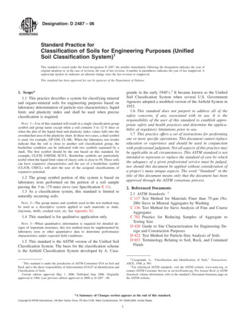
Author's personal copy1046Mach Learn (2017) 106:1039–10821aT1 xi b1aT1 xi b12aT2 xi b243aT2 xi b25aT3 xi b36aT3 xi b37Fig. 2 The maximal tree for depth D 2To see that the most natural representation for formulating the optimal decision tree problem (1) is using MIO, we note that at every step in tree creation, we are required to make anumber of discrete decisions:– At every new node, we must choose to either branch or stop.– After choosing to stop branching at a node, we must choose a label to assign to this newleaf node.– After choosing to branch, we must choose which of the variables to branch on.– When classifying the training points according to the tree under construction, we mustchoose to which leaf node a point will be assigned such that the structure of the tree isrespected.Formulating this problem using MIO allows us to model all of these discrete decisions in asingle problem, as opposed to recursive, top-down methods that must consider these decisionevents in isolation. Modeling the construction process in this way allows us to consider thefull impact of the decisions being made at the top of the tree, rather than simply making aseries of locally optimal decisions, also avoiding the need for pruning and impurity measures.We will next formulate the optimal tree creation problem (1) as an MIO problem. Considerthe problem of trying to construct an optimal decision tree with a maximum depth of D. Giventhis depth, we can construct the maximal tree of this depth, which has T 2(D 1) 1 nodes,which we index by t 1, . . . , T . Figure 2 shows the maximal tree of depth 2.We use the notation p(t) to refer to the parent node of node t, and A(t) to denote the setof ancestors of node t. We also define A L (t) as the set of ancestors of t whose left branchhas been followed on the path from the root node to t, and similarly A R (t) is the set ofright-branch ancestors, such that A(t) A L (t) A R (t). For example, in the tree in Fig. 2,A L (5) {1}, A R (5) {2}, and A(5) {1, 2}.We divide the nodes in the tree into two sets:Branch nodes Nodes t T B {1, . . . , ⌊T /2⌋} apply a split of the form aT x b. Points thatsatisfy this split follow the left branch in the tree, and those that do not follow the rightbranch.Leaf nodes Nodes t T L {⌊T /2⌋ 1, . . . , T } make a class prediction for each point thatfalls into the leaf node.We track the split applied at node t T B with variables at R p and bt R. We willchoose to restrict our model to univariate decision trees (like CART), and so the hyperplane123

Author's personal copyMach Learn (2017) 106:1039–10821047split at each node should only involve a single variable. This is enforced by setting theelements of at to be binary variables that sum to 1. We want to allow the option of notsplitting at a branch node. We use the indicator variables dt 1{node t applies a split} totrack which branch nodes apply splits. If a branch node does not apply a split, then we modelthis by setting at 0 and bt 0. This has the effect of forcing all points to follow the rightsplit at this node, since the condition for the left split is 0 0 which is never satisfied. Thisallows us to stop growing the tree early without introducing new variables to account forpoints ending up at the branch node—instead we send them all the same direction down thetree to end up in the same leaf node. We enforce this with the following constraints:p!j 1a jt dt , t T B ,(2)0 bt dt , t T B ,a jt {0, 1},(3)j 1, . . . , p, t T B ,(4)where the second inequality is valid for bt since we have assumed that each x i [0, 1] p , andwe know that at has one element that is 1 if and only if dt 1, with the remainder being 0.Therefore we it is always true that 0 aTt x i dt for any i and t, and we need only considervalues for bt in this same range.Next, we will enforce the hierarchical structure of the tree. We restrict a branch node fromapplying a split if its parent does not also apply a split.dt d p(t) , t T B P\{1},(5)z it lt , t T B ,(6)z it Nmin lt , t T B .(7)where no such constraint is required for the root node.We have constructed the variables that allow us to model the tree structure using MIO; wenow need to track the allocation of points to leaves and the associated errors that are inducedby this structure.We introduce the indicator variables z it 1{xi is in node t} to track the points assigned toeach leaf node, and we will then use the indicator variables lt 1{leaf t contains any points}to enforce a minimum number of points at each leaf, given by Nmin :n!i 1We also force each point to be assigned to exactly one leaf:!z it 1, i 1, . . . , n.(8)t T LFinally, we apply constraints enforcing the splits that are required by the structure of thetree when assigning points to leaves:aTm xi bt M1 (1 z it ), i 1, . . . , n, t T B , m A L (t),aTm xi(9) bt M2 (1 z it ), i 1, . . . , n, t T B , m A R (t),(10)Note that the constraints (9) use a stri

Mach Learn (2017) 106:1039-1082 DOI 10.1007/s10994-017-5633-9 Optimal classification trees Dimitris Bertsimas1 · Jack Dunn2 Received: 17 September 2015 / Accepted: 3 March 2017 / Published online: 3 April 2017 TheAuthor(s)2017 Abstract State-of-the-art decision tree methods apply heuristics recursively to create each