WIXLIB

The prime example of a linear time series is given by the aforementionedAuto-Regressive (AR) family pioneered by G. Yule [45] in which the timeseries {Yt } has a linear relationship with respect to its own lagged values,namelyYt p θk Yt k Zt(8)k 1with the error process {Zt } being i.i.d. as in eq. (5). AR modeling lends itselfideally to the problem of prediction of future values of the time series.For concreteness, let us focus on the one-step-ahead prediction problem,i.e., predicting the value of Yn 1 on the basis of the observed data Y1 , . . . , Yn ,and denote by Ŷn 1 the optimal (with respect to Mean Squared Error) predictor. In general, we can write Ŷn 1 gn (Y1 , . . . , Yn ) where gn (·) is anappropriate function. As can easily be shown [3], the function gn (·) thatachieves this optimal prediction is given by the conditional expectation, i.e.,Ŷn 1 E(Yn 1 Y1, . . . , Yn ). Thus, to implement the one-step-ahead prediction in a general nonlinear setting requires knowledge (or accurate estimation) of the unknown function gn (·) which is far from trivial [16] [43] [42].In the case of a causal AR model [8] however, it is easy to show that the function gn (·) is actually linear, and that Ŷn 1 pk 1 θk Yn 1 k . Note furthermore the property of ‘finite memory’ in that the prediction function gn (·)is only sensitive to its last p arguments. Although the ‘finite memory’ property is specific to finite-order causal AR (and Markov) models, the linearityof the optimal prediction function gn (·) is a property shared by all causallinear time series satisfying eq. (6); this broad class includes all causal andinvertible, i.e., “minimum-phase” [37], ARMA models with i.i.d. innovations.9

However, the property of linearity of the optimal prediction function gn (·)is shared by a larger class of processes. To define this class, consider a weakerform of (6) that amounts to relaxing the i.i.d. assumption on the errors tothe assumption of a martingale difference, i.e., to assume thatYt βi νt i(9)i 0where {νt } is a stationary martingale difference adapted to Ft , the σ-fieldgenerated by {Ys , s t}, i.e., thatE[νt Ft 1 ] 0 and E[νt2 Ft 1 ] 1 for all t.(10)Following [25], we will use the term weakly linear for a time series {Yt } thatsatisfies (9) and (10). As it turns out, the linearity of the optimal predictionfunction gn (·) is shared by all members of the family of weakly linear timeseries;3 see e.g. [36] and Theorem 1.4.2 of [20].Gaussian series form an interesting subset of the class of linear time series.They occur when the series {Zt } of eq. (5) is i.i.d. N(0, σ 2 ), and they tooexhibit the useful linearity of the optimal prediction function gn (·); to seethis, recall that the conditional expectation E(Yn 1 Y1, . . . , Yn ) turns out tobe a linear function of Y1 , . . . , Yn when the variables Y1 , . . . , Yn 1 are jointlynormal [8].Furthermore, in the Gaussian case all spectra of order higher than two areidentically zero; it follows that all dependence information is concentrated in3There exist, however, time series not belonging to the family of weakly linear seriesfor which the best predictor is linear. An example is given by a typical series of squaredfinancial returns, i.e., the series {Vt } where Vt Xt2 for all t, and {Xt } is modeled byan ARCH/GARCH model [25]. Other examples can be found in the class of randomcoefficient AR models [44].10

the spectral density f (w). Thus, the investigation of a Gaussian series’ dependence structure can focus on the simple study of second order properties,namely the ACF ρ(k) and/or the spectral density f (w). For example, an uncorrelated Gaussian series, i.e., one satisfying ρ(k) 0 for all k, necessarilyconsists of independent random variables.To some extent, this last remark can be generalised to the linear setting: ifa linear time series is deemed to be uncorrelated, then practitioners typicallyinfer that it is independent as well.4 Note that to check/test whether an estimated ACF, denoted by ρ̂(k), is significantly different from zero, the Bartlettconfidence limits are typically used—see e.g. the bands in Figure 2 (a); butthose too are only valid for linear or weakly linear time series [17] [20] [38].To sum up: all the usual statistical goals of prediction, confidence intervals and hypothesis testing are greatly facilitated in the presence of linearity,and particularly in the presence of normality.Linearising or normalising the stock market?It should come as no surprise that a simple parametric model as (1) mightnot perfectly capture the behavior of a complicated real-world phenomenonsuch as the evolution of financial returns that—almost by definition of market‘efficiency’—ranks at the top in terms of difficulty of modeling/prediction. Asa consequence, researchers have recently been focusing on alternative modelsfor financial time series.4Strictly speaking, this inference is only valid for the aforementioned class of causaland invertible ARMA models [6].11

For example, consider the modelXt σ(t) Zt(11)where Zt is i.i.d. (0, 1). If {σ(t)} is considered a random process independentof {Zt }, then (11) falls in the class of stochastic volatility models [40]. If,however, σ(·) is thought to be a deterministic function that changes slowly(smoothly) with t, then model (11) is nonstationary—although it is locallystationary [11]—, and σ(·) can be estimated from the data using nonparametric smoothing techniques; see e.g. [21] and the references therein.As another example, consider the nonparametric ARCH model definedby the equation:Xt gp (Xt 1 , . . . , Xt p ) Zt(12)where Zt is i.i.d. (0, σ 2 ), and gp is an unknown smooth function to be estimated from the data. Additional nonparametric methods for financial timeseries are discussed in the review paper [15].Despite their nonparametric (and possibly nonstationary) character, theabove are just some different models attempting to fully capture/describethe probabilistic characteristics of a financial time series which is perhaps anoverly ambitious task. Foregoing the goal of finding the ‘best’ model, we mayinstead resort to an exploratory, model-free approach in trying to understandthis difficult type of data. In particular, we may attempt to transform theproblem into a more manageable setting such as the setting of linearity.Consider again the financial returns data Xn (X1 , . . . , Xn ), and a transformation of the type Vn H(Xn ) where Vn is also n-dimensional. Ideally,12

we would like the transformed series Vn (V1 , . . . , Vn ) to be linear since, asmentioned before, such time series are easy to work with.However, just asking for linearity of the transformed series is not enough.For example, the naive transformation Vt sign(Xt ) may be thought of as alinearising transformation since, by the efficient market hypothesis, sign(Xt )is i.i.d. (taking the values 1 and -1 with equal probability), and thereforelinear. Nevertheless, in spite of the successful linearisation, the sign transformation is not at all useful as the passage from Xn to Vn is associated witha profound loss of information.To avoid such information loss “due to processing” [10], we should furtherrequire that the transformation H be in some suitable sense invertible, allowing us to work with the linear series Vt but then being able to recapture theoriginal series by the inverse transformation H 1 (Vn ). Interestingly, the keyto finding such a transformation is asking for more: look for a normalising(instead of just linearising) information preserving transformation.We now show how this quest may indeed be fruitful using the ARCHequation (1) as a stepping stone. Note that eq. (1) can be re-written asZt a Xt pi 12ai Xt i.Hence, we are led to define the trasformed variable Vt byVt Xt 2αs2t 1 a0 Xt2 pi 1 ai Xt ifor t p 1, p 2, . . . , n,(13)and Vt Xt /st for t 1, 2, . . . , p. In the above, α, a0 , a1 , . . . , ap are non2 V ar(X1 )negative real-valued parameters, and s2t 1 is an estimator of σXbased on the data up to (but not including) time t. Under the zero mean t 1 2Xk .assumption for Xt , the natural estimator is s2t 1 (t 1) 1 k 113

The invertibility of the above transformation is manifested by solvingeq. (13) for Xt , thus obtaining: p Vt2 αs2 ai Xt iXt t 121 a0 Vti 1for t p 1, p 2, . . . , n. (14)Given the initial conditions X1 , . . . , Xp , the information set FnX {Xt , 1 t n} is equivalent to the information set FnV {Vt , 1 t n}. Tosee this, note that with eq. (14) we can recursively re-generate Xt for t p 1, p 2, . . . , n using just FnV and the initial conditions; conversely, eq.(13) defines Vt in terms of FnX .Equation (13) describes the candidate normalising (and therefore also linearising) transformation, i.e., the operator H in Vn H(Xn ); this transformation was termed ‘NoVaS’ in [31] which is an acronym for Normalizing andVariance Stabilising. Note that formally the main difference between eq. (13)and the ARCH eq. (1) is the presence of the term Xt2 paired with the coefficient a0 inside the square root; this is a small but crucial difference withoutwhich the normalisation goal is not always feasible [29] [31]. A secondary difference is having αs2t 1 take the place of the parameter a; this is motivatedby a dimension (scaling) argument in the sense that choosing/estimating αis invariant with respect to a change in the units of measurement of Xt . Suchinvariance does not hold in estimating the parameter a in eq. (1).Despite its similarity to model (1), eq. (13) is not to be interpreted as a“model” for the {Xt } series. In a modeling situation, the characteristics of themodel are pre-specified (e.g., errors that are i.i.d. N(0, σ 2 ), etc.), and standardmethods such as Maximum Likelihood or Least Squares are used to fit themodel to the data. By contrast, eq. (13) does not aspire to fully describe14

the probabilistic behavior of the {Xt } series. The order p and the vector ofnonnegative parameters (α, a0, . . . , ap ) are chosen by the practitioner withjust the normalisation goal in mind, i.e., in trying to render the transformedseries {Vt } as close to normal as possible; here, ‘closeness’ to normality canbe conveniently measured by the Shapiro-Wilk (SW) test statistic [39] or itscorresponding P -value.It is advantageous (and parsimonious) in practice to assign a simple structure of decay for the ak coefficients. The most popular such structure—sharedby the popular GARCH(1,1) model [4]—is associated with an exponentialrate of decay, i.e., postulating that ak Ce dk for some positive constantsd and C which—together with the parameter α—are to be chosen by thepractitioner.Taking into account the convexity requirementα ak 1,k 0the exponential coefficients scheme effectively has only two free parametersthat can be chosen with the normalisation goal in mind, i.e., chosen to maximise the SW statistic calculated on the transformed series Vt or linear combinations thereof—the latter in order to also ensure normality of joint distributions.As it turns out, the normalisation goal can typically be achieved by a greatnumber of combinations of these two free parameters, yielding an equallygreat number of possible normalising transformations. Among those equallyvalid normalising transformations the simplest one corresponds to the choiceα 0. Alternatively, the value of α may be chosen by an additional op15

3210-1normalised SP500-2-3050010001500200025003000timeFigure 3: Normalised S&P500 returns, i.e., the tranformed V -series, spanningthe same period 8-30-1979 to 8-30-1991.timisation criterion driven by an application of interest such as predictiveability.For illustration, let us revisit the S&P500 returns dataset. The normalising trasformation with ak Ce dk and the simple choice α 0 is achievedwith d 0.0675; the resulting tranformed V -series is plotted in Figure 3which should be compared to Figure 1. Not only is the phenomenon ofvolatility clustering totally absent in the tranformed series but the outlierscorresponding to the crash of October 1987 are hardly (if at all) discernible.Quantifying nonlinearity and nonnormalityThere are many indications pointing to the nonlinearity of financial returns.For instance, the fact that returns are uncorrelated but not independent is16

a good indicator; see e.g. Figure 2 (a) and (b). Notably, the ARCH modeland its generalisations are all models for nonlinear series.To quantify nonlinearity, it is useful to define the new functionK(w1 , w2) F (w1 , w2) 2.f (w1)f (w2 )f (w1 w2 )(15)From eq. (7), it is apparent that if the time series is linear, then K(w1 , w2 )is the constant function—equal to µ23 /(2πσ 6) for all w1 , w2 ; this observationcan be used in order to test a time series for linearity [22] [41]; see also [23][24] and [26] for an up-to-date review of different tests for linearity.5 In theGaussian case we have µ3 0 and therefore F (w1 , w2 ) 0 and K(w1 , w2 ) 0as well.Let K̂(w1 , w2 ) denote a data-based nonparametric estimator of the quantity K(w1 , w2 ). For our purposes, K̂(w1 , w2 ) will be a kernel smoothed estimator based on infinite-order flat-top kernels that lead to improved accuracy[33]. Figure 4 shows a plot of K̂(w1 , w2 ) for the S&P500 returns; its nonconstancy is direct evidence of nonlinearity. By contrast, Figure 5 showsa plot of K̂(w1 , w2 ) for the normalised S&P500 returns, i.e., the V -series.Note that, in order to show some nontrivial pattern, the scale on the verticalaxis of Figure 5 is 500 times bigger than that of Figure 4. Consequently, thefunction K̂(w1 , w2 ) for the normalised S&P500 returns is not statistically different from the zero function, lending support to the fact that the trasformedseries is linear with distribution symmetric about zero; the normal is such adistribution but it is not the only one.5A different—but related—fact is that the closure of the class of linear time series islarge enough so that it contains some elements that can be confused with a particular typeof nonlinear time series; see e.g. Fact 3 of [2].17

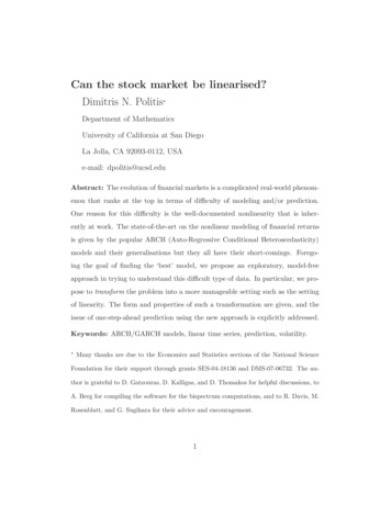
Figure 4: ABOUT HEREFigure 5: ABOUT HERETo further delve into the issue of normality, recall the aforementionedShapiro-Wilk (SW) test which effectively measures the lack-of-fit of a quantilequantile plot (QQ-plot) to a straight line. Figure 6 shows the QQ-plot of theS&P500 returns; it is apparent that a straight line is not a good fit. Asa matter of fact the SW test yields a P-value that is zero to several decimal points—the strongest evidence of nonnormality of stock returns. Bycontrast, the QQ-plot of the normalised S&P500 returns can be very wellapproximated by a straight line: the R2 associated with the plot in Figure 7is 0.9992, and the SW test yields a P-value of 0.153 lending strong support tothe fact that the trasformed series is indistiguishable from a Gaussian series.The proposed transformation technique has been applied to a host of different financial datasets including returns from several stock indices, stockprices and foreign exchange rates [34]. Invariably, it was shown to be successful in its dual goal of normalisation and linearisation. Furthermore, as already discussed, a welcome by-product of linearisation/normalisation is thatthe construction of out-of-sample predictors becomes easy in the transformedspace.Of course, the desirable objective is to obtain predictions in the original(untransformed) space of financial returns. The first thing that comes tomind is to invert the transformation so that the predictor in the transformedspace is mapped back to a predictor in the original space; this is indeed possible albeit suboptimal. Optimal predictors were formulated in [31], and are18

0.050.0-0.05data quantiles-0.10-0.15-0.20-202normal quantilesFigure 6: QQ-plot of the S&P500 returns.described in the Appendix where the construction of predictive distributionsis also discussed.Notably, predictors based on the NoVaS transformation technique havebeen shown to outperform GARCH–based predictors in a host of applicationsinvolving both real and simulated data [31] [34]. In addition, the NoVaSpredictors are very robust, performing well even in the presence of structuralbreaks or other nonstationarities in the data [35]. Perhaps the most strikingfinding is that with moderately large sample sizes (of the order of 350 dailydata), the NoVaS predictors appear to outperform GARCH–based predictorseven when the underlying data generating process is itself GARCH [35].19

3210data quantiles-1-2-3-202normal quantilesFigure 7: QQ-plot of the normalised S&P500 returns.Appendix: Prediction via the transformation techniqueFor concreteness, we focus on the problem of one-step ahead prediction, i.e.,prediction of a function of the unobserved return Xn 1 , say h(Xn 1 ), basedon the observed data FnX {Xt , 1 t n}. Our normalising transformationaffords us the opportunity to carry out the prediction in the V -domain wherethe prediction problem is easiest since the problem of optimal predictionreduces to linear prediction in a Gaussian setting.The prediction algorithm is outlined as follows: Calculate the transformed series V1 , . . . , Vn using eq. (13). Calculate the optimal predictor of Vn 1 , denoted by V̂n 1 , given FnV . q 1This predictor would have the general form V̂n 1 i 0ci Vn i. Theci coefficients can be found by Hilbert space projection techniques, or20

by simply fitting the causal AR modelVt 1 q 1 ci Vt i t 1 .(16)i 0to the data wheretis i.i.d. N(0, σ 2 ). The order q can be chosen byan information criterion such as AIC or BIC [9].Note that eq. (14) suggests that h(Xn 1 ) un (Vn 1 ) where un is given by p V2 αs2 .ai Xn 1 iun (V ) h t 121 a0 Vi 1Thus, a quick-and-easy predictor of h(Xn 1 ) could then be given by un (V̂n 1 ).A better predictor, however, is given by the center of location of the distribution of un (Vn 1 ) conditionally on FnV . Formally, to obtain an optimalpredictor, the optimality criterion must first be specified, and correspondingly the form of the predictor is obtained based on the distribution of thequantity in question. Typical optimality criteria are L2 , L1 and 0/1 losseswith corresponding optimal predictors the (conditional) mean, median andmode of the distribution. For reasons of robustness, let us focus on themedian of the distribution of un (Vn 1) as such a center of location.Using eq. (16) it follows that the distribution of Vn 1 conditionally on FnVis approximately N(V̂n 1 , σ̂ 2 ) where σ̂ 2 is an estimate of σ 2 in (16). Thus,the median-optimal one-step-ahead predictor of h(Xn 1 ) is the median ofthe distribution of un (V ) where V has the normal distribution N(V̂n 1 , σ̂ 2 ) truncated to the values 1/ a0 ; this median is easily computable by MonteCarlo simulation.The above Monte-Carlo simulation actually creates a predictive distribution for the quantity h(Xn 1 ). Thus, we can go a step further from the21

notion of a point-predictor: clipping the left and right tail of this predictivedistribution, say δ·100% on each side, a (1 2δ)100% prediction intervalfor h(Xn 1 ) is obtained. Note, however, that this prediction interval treatsas negligible the variability of the fitted parameters α, a0 , a1 , ., ap which isa reasonable first-order approximation; alternatively, a bootstrap methodmight be in order [28] [32].References[1] Bachélier, L. (1900).

Can the stock market be linearised? Dimitris N. Politis Department of Mathematics University of California at San Diego La Jolla, CA 92093-0112, USA e-mail: dpolitis@ucsd.edu Abstract: The evolution of financial markets is a complicated real-world phenom-enon that ranks at th