Transcription
Quantum ComputingMarija Kranjčević, Filip Kiršek, Petar KunštekAbstractThis paper explains the basics of quantum computing and gives an overview of someof the more notable quantum algorithms, such as Grover’s search algorithm and Shor’sfactoring algorithm.1IntroductionThere are many formulations of the Moore’s law, but they all converge upon a similar conclusion: the performance of the computer chips increases, while the size decreases exponentiallyover time. This growth is obviously unsustainable; the classical physical models used in theconstruction of current computers cease to be a satisfying approximation at atomic and subatomic levels. This alone should be enough for one to be interested in quantum computing.There is more to it than that, however. Problems unsolvable through increase of computingpower alone (e.g. factoring a large number within the current cycle of the universe) can besolved on quantum computers, using quantum algorithms (e.g. Shor’s factoring algorithm).The downside is that quantum physics and, by extension, quantum computing often seemesoteric. This paper hopes to provide some insight into this potentially interesting field ofresearch. It should not be consulted as a definitive guide to quantum computing, but as anintroduction to the subject, providing a brief overview of the physical principles, the mathematical model and a somewhat more in-depth overview of the more important quantumalgorithms. The number theory definitions and theorems used in the explanations of thesealgorithms are presented in Appendix.2Results From Quantum Physics(by Petar Kunštek)Studying quantum physics is probably not as hard as it is confusing and unintuitive. Themain reason is that, on many levels, quantum physics differs from classical physics. The“intuitive” models from classical physics usually can not be applied to explain quantumeffects.A similar situation is encountered when comparing relativistic and non-relativistic systems.There is no need for a relativistic model if an object’s speed is small in comparison with thespeed of light, c1 ; the classical theory is a satisfying approximation. But, when the object’sspeed approaches c, classical theory differs greatly from the actual results.The same principle exists in differing between quantum and classical approach. In this case,1c 3 · 108 m/s1
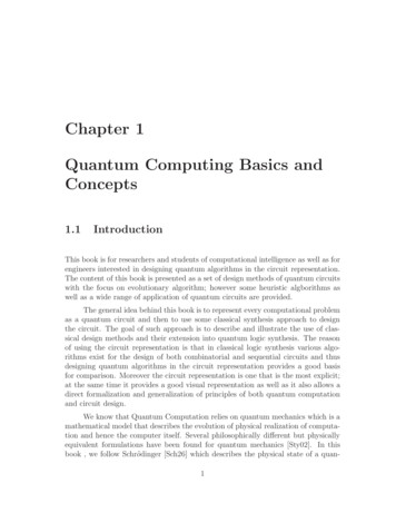
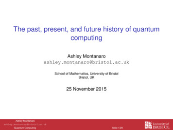
the constant defining the scales at which classical theory becomes inapplicable is the Planckconstant2 , denoted h. Therefore, particles at the atomic scales (less than 100 nm), can beseen to exhibit some unintuitive properties.2.1Quantum SuperpositionMirror experimentPerhaps the best way to demonstrate this unintuitive property is an experiment. Let’s takea source of light, two sensors and one half-silvered mirror, arranged like in Figure 1. Thestarting assumption is that a photon may be reflected or transmitted through the halfsilvered mirror with the same probability. That is indeed the result of such an experiment:both sensors, measuring the intensity of light, detect the same level of intensity.Figure 1: Half-silvered mirrorNow, with that hypothesis, complex structures of half-silvered and silvered mirrors can beconstructed. Let us take two silvered mirrors (where total reflection occurs), two half-silveredmirrors, two sensors, denoted A and B, and a source of light, and arrange them as shownin Figure 2. Intuitively, it is expected that sensor A and sensor B each detect 50% of lightintensity. Considering that a photon has a 50% chance to be reflected or transmitted, thereshould be four different possible paths, each occurring with the probability of 25%. Becausetwo of those paths lead to sensor A, and the other two to sensor B, it could be expectedthat a photon has an equal chance of hitting each sensor. Yet, the experiment results aredrastically different.Sensor A constantly detects 100% of light intensity, while sensor B detects nothing. Howto explain this phenomenon? Imagine that, instead of a small ball, a photon is a wave. Ifa single photon is studied in more detail, one could assume that, when it approached thefirst half-silvered mirror, the photon didn’t “decide” which path to take, but reflected anttransmitted at the same time. Thus, at point S, the photon as wave is found in both ofthese states (created by two different paths) and, one could conclude that, toward sensor A2h 6.626 · 10 34 Js2
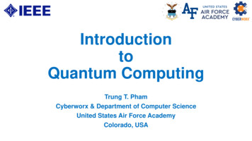
Figure 2: Mirror experimentthe photon is in a constructive interference and toward sensor B in destructive interference.Consequently, sensor A is always detecting photons, while sensor B detects nothing.This is called superposition of waves. The real surprise is the fact that all particles can actas waves. As a result, small particles (e.g. electrons) don’t posses the expected corporealeffects. The presented idea was first introduced by de Broglie3 at the beginning of thetwentieth century.2.2The Measuring PrincipleLet us modify our experiment by placing a sensor device, which detects whether or not ourphoton passed through it, in one possible path (Figure 3).The results of this modified experiment are actually the expected results of the originalexperiment. This demonstrates that, when a quantum system is measured (i.e. some information is obtained) quantum superposition ceases to exist. The system is then forced to“choose” between all possible results (in this case two paths) and behaves correspondinglyfrom that point on.2.3Quantum EntanglementConsider a collision between two particles. Such collisions can produce new particles, solet us assume an electron and a positron4 were produced as a result of one such collision.There exists an experiment that determines the spin of the electron, and it can only obtaintwo results: up or down. If the electron is measured to have a certain spin (e.g. spin up),any measurement on the positron will produce the opposite result (in this case, down spin).3 LouisVictor de Broglie (1892.-1987.), French physicistpossessing positive electric charge, counterpart to electron4 antiparticle3
Figure 3: Mirror experiment with photon path detectionThis phenomenon is one example of quantum entanglement.To further explain quantum entanglement, let us consider another thought experiment.Popper’s experimentPopper’s5 experiment is based on the uncertainty principle, i.e. the fact that, for a givenparticle, the uncertainty of momentum is inversely proportional to the uncertainty of position. In other words, if an object’s position is well known, momentum is very uncertain,and vice versa. As in the previous example, let us take a source of particles, which createsthem in pairs, as a result of collision. Let there also be two walls with narrow slits and away to determine the momentum of the exiting particle (Figure 4).To simplify, imagine a creation of a single pair where particles are moving in the oppositedirections (which is actually a necessity in physics), one moving through slit A and anotherthrough slit B. In this case, both sensors would measure the same uncertainty. But, let’snow change the size of the slit on wall A so that it is considerably bigger, but still smallenough so that the sensor is able to detect the uncertainty in momentum. By applying theuncertainty principle, one may conclude that the uncertainty of momentum on the sensorA should be smaller than the uncertainty of momentum on the sensor B. But, the resultsare, rather surprisingly, the same, meaning that sensor A isn’t able to detect any higher uncertainty. This can be explained through quantum entanglement. As one pair was passingthrough the slit on the wall B, information about the uncertainty of position became thesame for both particles (although the particle moving toward wall A was passing through abigger slit), resulting in both particles having the same uncertainty in momentum.5 SirKarl Raimund Popper (1902.-1994.), Austro-British philosopher4
Figure 4: Popper’s experiment3The Mathematical Model(by Filip Kiršek)As was shown in the previous section, quantum physics deals with some unusual phenomena,most importantly, superposition, the influence of measurement on the observed system, andquantum entanglement. These properties of quantum systems are used as a basis in theconstruction of both the mathematical model of a quantum computer and the computeritself. A well-defined mathematical model allows us to solve problems unsolvable using themodel for the classical computer.63.1QubitsBit is a basic unit of information in classical computing. The entirety of classical computingis based on finite sequences of bits and manipulations thereof. Qubit, its quantum analogue,has a similar role in quantum computing.Suppose that we know a bit has a value 1. Depending on where the bit “resides”, the harddrive or the processor, that might mean that there is a non-zero current through a wire orthat a part of the hard drive is magnetized. Similarly, an electron might be measured havingeither an up spin or a down spin. Electron, however, exhibits other properties that make itill-fitting to be considered a bit.Qubit is defined as a 2-dimensional complex vector, an element of C2 . Two base statestare denoted as 0i and 1i, and they are represented by base state vectors, 0i (1, 0) ,tand 1i (0, 1) , 0i, 1i C2 . Results from the theory of quantum physics tell us thatquantum-mechanical systems rarely behave discreetly but are rather superpositions of themany possible states. Therefore, before measurement, qubit is in a superposition of 0i and 1i. This means that any other qubit is a linear combination of base states, φi α 0i β 1i, with the constraint that α 2 β 2 1 (where for α a bi, a, b R, α a2 b2 ).This normalization constraint is a result of the meaning behind α and β. α 2 representsthe probability of obtaining 0i when measuring our qubit and β 2 , likewise, represents theprobability of measuring 1i.The i is called a “ket”, and, as was shown above, represents vectors, not just base statevectors. Generally speaking, kets represent qubits. For every ket, there is also a “bra”, which6 mostof the definitions presented in this section were obtained from [3] and [4]5
can be interpreted as a row vector or, more precisely, a linear operator of scalar product. Inother words, for ψi α 0i β 1i, the corresponding bra is: hψ α h0 β h1 (α , β ),or, more precisely, hψ : C2 C2 , hψ (x) hhψ , xi 7 . Later on, we will use simply hx yi,and this is called a “braket”.3.2MeasurementMeasurement of qubits is an important part of any quantum algorithm. As mentioned before,measuring quantum-mechanical systems alters them. When measuring a single qubit, weare actually collapsing the superposition and obtaining one of the base states, depending onthe amplitudes (a measurement of ψi α 0i β 1i will give 0i with the probability α 2and 1i with the probability β 2 ).In the context of quantum computing, after measuring our ψi, we collapse its superpositionand it becomes either 0i or 1i, and, from that point on, it will behave correspondinglywithin the algorithm. Were we to measure the same qubit two or more times consecutively,all the measurements would give the same result as the first one. Any transformations overa qubit after it is measured will behave as if the qubit is in one of the base states - which itis. This is the reason that many quantum algorithms simply discard the measured qubit.One might think that using qubits is a far more effective storage solution than the standardbit. The entirety of human knowledge, one might say, can be stored in the segment [0,1], so,logically, we would need but one qubit to derive wondrous amounts of information. This,however, misses one key property of qubits: during measurement, we only detect 0i or 1i,depending on the probabilities associated with that qubit. To obtain just the norms of theamplitudes one must measure the same qubit infinitely many times. Even then, throughmeasurement alone, we cannot differentiate between 0i and i 0i.The other reason why a qubit is not a better information storage than the bit is that wecannot copy qubits, or any quantum system, since copying it would involve measuring it,which would collapse the superposition and render the whole process useless.8The question as to why something with two base states is chosen instead of three or moremay also arise. Those systems are also a possibility - systems with three base states arecalled qutrits, but, like its classical origin point trit, qutrit isn’t widely used, partly becauseof simplicity and partly because we already have a solid basis in bits. Therefore, we willonly deal with qubits.3.3Bloch sphereLet us observe a given qubit of the form ψi α 0i β 1i where α, β C, α 2 β 2 1. Itcan be easily shown that there exists a c C such that c 1 and c ψi α0 0i β 0 1i, whereα0 R, α0 0. This can be written as c ψi cos θ2 0i eiφ sin θ2 1i, for some φ, θ R.Qubits ψi and c ψi are indistinguishable through measurement and any combination ofquantum gates, which we will define later on. This means that we can treat any qubit asbeing equal to cos θ2 0i (cos φ i sin φ) sin θ2 1i, where θ [0, π], φ [0, 2π], producing amap from the set of qubits onto a unit sphere, where we treat θ and φ as polar coordinates(Figure 5a).7 α 8arepresents the complex conjugate of α, , is the standard scalar product in C2more detailed reasoning can be found in [4]6
The poles of the Bloch sphere represent 0i and 1i. Any two orthogonal qubits are joinedto antipodal points of the Bloch sphere (Figure 5b). Therefore, any two antipodal pointsrepresent a single orthogonal basis.Figure 5: a) Bloch sphere, b) Orthogonal qubits on the Bloch sphere3.4Quantum registersIntuitively, given two qubits x and y, since both x and y can be measured in two possiblestates, the quantum register containing only x and y has 4 possible states. We thereforedenote the (new) base states as 00i, 01i, 10i, 11i9 , and all possible register states arelinear combinations of these base states with complex coefficients. The two-qubit system istherefore constructed within C4 . To do that, we use the standard tensor product. To recap(without the usual mathematical rigour), the tensor product from two 2-dimensional vectorspaces is: (x, y)t (z, w)t (xz, xw, yz, yw)t , and the general tensor product : Ck Cl Ckl is defined with: v1 w . . kl v w : vj w , v C , w C , . . vk wwhere vj is the j-th component of vector v. Ckl can, therefore, be constructed using thetensor product on all base vectors. It is obvious that our n-qubit system is contained in the9 base states in a two-qubit system are sometimes denoted 0i, 1i, 2i, 3i (etc. for systems with more thantwo qubits); this plays a role in some algorithms where the input might be a natural number n representedprecisely by the n-th base state of that quantum register7
nvector space C2 .The definition of the tensor product is easily extended to matrices, which plays a vital rolein constructing multi-qubit quantum gates.Using the tensor product, we can easily combine qubits into elements of the extended system.Indeed, { 0i, 1i} { 0i, 1i} is the standard basis for C4 , where 0i 0i 00i, 1i 0i 10ietc., and similarly for an arbitrary quantum registerSince our quantum register also represents a quantum system and the amplitudes provideus with probabilities, it is obvious that we have to generalize the restriction regarding theamplitudes in a single qubit system: the norm of our quantum register (when we considerit to be a vector in Cn ) must be equal to 1. In other words:Pn any given quantum register ψi α1 00.0i . αn 11.1i must satisfy the equation k 1 αk 2 1, where αk 2 is theprobability of measuring the corresponding base state when measuring the entire quantumregister. As demonstrated, this is a natural generalization of a single qubit system discussedpreviously and many of the properties remain unchanged.3.5Entangled QubitsConsider a quantum register defined with ψi 12 00i 12 10i 12 11i. When measuringthe first qubit of this quantum register, if the measurement gives us 0i, the second qubitalso collapses completely, since the only possible measurement result for the second qubit isobviously 0i. On the other hand, were we to measure 1i on the first qubit, our quantumregister would transform into ψi 12 10i 12 11i, which, when measuring the secondqubit, has the same probability of giving 0i and 1i, while, originally, it was somewhat moreprobable to measure 0i. (Note: we also had to resize the amplitudes to conserve the normof our two-qubit register.)Conversely, consider φi 12 00i 12 01i 21 10i 12 11i. It is evident that the result of anymeasurement of the state of the first qubit won’t influence the results of measurement overthe second qubit.It can be easily shown that measurement over an individual qubit won’t influence the remaining qubits if and only if the quantum register can be described as a direct tensor productof that qubit and the remaining multi-qubit vector.When we also take into consideration that measurement changes the behaviour of that system, meaning that even a partial measurement can alter the behaviour of our quantumregister, we can see that this effect corresponds to the physical effect of quantum entanglement. Indeed, this is one of the justifications for our model. This produces the followingdefinition: A multi-qubit state is entangled if it cannot be factored into a direct product ofindividual qubits.Entanglement is an interesting property since, given two or more entangled qubits, transformations over one qubit affect the entire register. This will play a crucial role in manyquantum algorithms.3.6Quantum gatesHaving defined qubits and quantum registers, it is now time to introduce the way we manipulate them. Firstly, it is obvious that any manipulation over a qubit or a quantum registermust retain the norm. Furthermore, given that we are operating over superpositions, our8
transformations will be defined over base states and the definition expanded for an arbitraryqubit through linearity of the transformation. These conditions gives us our definition:A quantum gate is a unitary transformation.NOT - gateLet us consider the classical logical NOT gate. Its purpose is simple: it maps 0 to 1 and 1to 0. Using that as a starting point for constructing the quantum NOT gate, it is obviousthat we have our work cut out for us; since we already know that 0i 1i and conversely 1i 0i, the quantum NOT - gate representation in matrix form is: 0 1X 1 0This gate is also often called Pauli-X gate since it corresponds to the rotation of a point onthe Bloch sphere by π radians around the X-axis. There are also Pauli-Y and Pauli-Z gatesrepresented as: 0 i1 0,Y , and Z i 00 1respectively.Hadamard gateThe Hadamard gate is deceptively simple; it is represented as 11 1,H 1 12when dealing with a singular qubit. This allows us to transform both 0i and 1i into statesthat have equal probabilities of measuring both base states. We can prepare the quantumregister in base states, and apply the Hadamard gate to each individual qubit to obtaina state that has equal probability of being measured in every single base state possible; auseful trick, and the reason most quantum algorithms contain the Hadamard gate.Its generalisation on the n-dimensional quantum register is defined recursively with 1Hn 1 Hn 1Hn ,Hn 1 Hn 12and it can be shown that this corresponds to applying the Hadamard transform to eachindividual qubit (if, of course, n 2m , for m N representing the number of qubits in thatregister).It should also be noted that the Hadamard transform is its own inverse - applying theHadamard gate twice to the same quantum register would leave the register unchanged.Phase-shift gateFor a given θ, a phase-shift gate is defined as: 1Θ 090eiθ
This corresponds to the mapping of 0i to 0i and 1i to eiθ 1i. It leaves the probabilities ofmeasuring 0i or 1i unchanged, but still makes a detectable change in the qubit.Applying, consecutively, the Hadamard gate, the θ phase shift gate, the Hadamard gate(again) and the π2 φ gate on 0i, we obtain a qubit in the phase cos θ2 0i eiφ sin θ2 1i(Figure 6).This, combined with the results given in the section 3.3, means that we can construct anyθ0HH𝜋 𝜙2cos𝜃20 𝑒 𝑖𝜙 sin𝜃21Figure 6: Construction of an arbitrary qubitunitary trasformation over a single qubit using only Hadamard and phase shift gates.CU gateControlled gates are common in classical computing; we may or may not want to perform atransformation over a given memory register, and we control that using some other memoryregister, usually a single bit.Given an arbitrary unitary transformation U over a single qubit: x1 x2U x3 x4a CU gate is constructed as: 1 0 CU 00010000x1x3 00 x2 x4This transformation corresponds precisely to a transformation in which the first qubit is leftunchanged and the other is unchanged when the first is 0i and changed by the transformation U if the first is 1i. This transformation, of course, works even when the first qubit isin neither of these base states.Quantum Fourier TransformWe will not discuss the importance of the Fourier transform in mathematics, nor explain itsusage. This section will give but a brief definition of the Quantum Fourier transform, whichwill later be used in quantum algorithms.10
QFT can be defined simply through its matrix as: 1112 1ωω 24 1ωωQF T . .1 ω N 1 ω 2(N 1).1 ω N 1ω 2(N 1). , ω (N 1)(N 1)where N is the dimension of the complex vector space (N 2n when dealing with the2πiregister of n qubits), and ω e N .PN 1This will map an arbitrary quantum register in the state φi k 0 xk ki toN 1Xk 04N 11 X yk ki, where yk xj ω jk .N j 0Quantum algorithms4.1(by Marija Kranjčević)Deutsch’s AlgorithmDeutsch’s10 algorithm is a very simple, deterministic11 algorithm, which solves a somewhatcontrived problem:Given a function f : {0, 1} {0, 1}, determine if f is balanced (i.e. if f (0) 6 f (1)) or constant (f (0) f (1)).A trivial solution, which can be carried out by any classical computer, is to compute bothf (0) and f (1) and compare them. However, using the fact that a quantum system canbe in several states simultaneously, a quantum computer produces a result with only oneevaluation of the given function.In a classical system, evaluating the function f would correspond to performing the operation which maps x to f (x). However, an arbitrary function f doesn’t have to be aunitary operation, whereas the operations performed on quantum states must be unitary.Therefore, to evaluate f on a quantum system, it is necessary to have a quantum gatewhich can be easily constructed from the function f . Such an operator can be defined withUf ( xi yi) xi y f (x)i, where is the exclusive operation (XOR). It is easy to see thatUf 1 Uf and that Uf is a unitary operator. Note: the input of the quantum algorithm isonly the black-box12 unitary operator Uf .The steps of Deutsch’s algorithm are as follows (Figure 7):1. Take two qubits, in states 0i and 1i, respectively. It is obvious that ϕ0 i 0, 1i.10 DavidElieser Deutsch (1953.-), Israeli-British physicistgives the correct answer.12 A device or theoretical construct whose inputs and outputs can be known, but there is no informationabout its internal structure.11 Always11
φ0φ2φ1Hφ3HUfHFigure 7: Deutsch’s algorithm2. Apply the Hadamard gate to both qubits to put them in a superposition of states.The state is now ϕ1 i 0i 1i 0i 1i 0, 0i 0, 1i 1, 0i 1, 1i .2223. Apply Uf to get 0, 0i 0, 1i 1, 0i 1, 1i)2 0, 0 f (0)i 0, 1 f (0)i 1, 0 f (1)i 1, 1 f (1)i 2 0, f (0)i 0, f (0)i 1, f (1)i 1, f (1)i ,2 ϕ2 i Uf (where, for x {0, 1}, xi denotes the opposite value of xi.This can be compactly written as( 1)f (0) 0i ( 1)f (1) 1i 0i 1i ϕ2 i [][ ]22( 0i 1i ( ) 0i 1iif f is constant,22 0i 1i 0i 1i ( ) 2if f is balanced.24. Apply the Hadamard gate to the first qubit. The state of the system becomes( ( ) 0i 0i 1iif f is constant,2 ϕ3 i 0i 1i( ) 1i 2if f is balanced.5. Measure the state of the first qubit. The measured result gives the solution of theinitial problem. If it is in the state 0i, then f is a constant function; otherwise, f is abalanced function.12
A quantum system allows for all the needed computations to be done in parallel, so multipleresults can be obtained by a single evaluation. This approach shows that, with a littlemanipulation to obtain a useful result, quantum algorithms, and quantum computers, cansolve certain problems much faster than their classical counterparts. Basically, while thesolution to this problem is not a very useful one, it shows the possibility of the use ofquantum computers and the main idea how the properties of quantum-mechanical systemscan be used to speed-up the solutions to some problems.134.2Grover’s AlgorithmAnother quantum algorithm is Grover’s14 algorithm for searching an unstructured database.Using classical computation, that problem cannot be solved in less than linear time, i.e.searching through every item. But, while classical algorithms need to successively test theindices, a quantum algorithm can test several indices at once, using quantum parallelism.Therefore, Grover’s algorithm is much faster and performs the search of a database with Nentries in only O( N ) steps.The problem of searching an unstructured database can be stated as follows:Take an unstructured database with N entries with indices in the range from 0to N 1. Suppose one of these element is tagged, i.e. let there be a black boxfunction ft , for some fixed t in the range from 0 to N 1, such that, for everyindex x, ft (x) δxt . The task is to find the index t using the fewest calls to thefunction ft .For simplicity, it can be assumed that N 2n , for some natural number n (if that is notthe case, a register of n dlog2 N e qubits can be used). The algorithm then requires aregister of n qubits to represent the indices of the database entries. (Also, a second register,consisting of a single qubit, is needed for constructing the gates.)The idea of Grover’s algorithm is to put the first register into an equal superposition ofall indices, and then gradually increase the amplitude of the searched-for index t. Thus, ameasurement after a certain number of steps is likely to give the index t.The steps of the algorithm are as follows15 (Figure 8):1. Set the first register to si 1NNP 1 xi.x 02. Use the function ft to construct a black box unitary operator Ut , which acts asUt ( xi) ( 1)ft (x) xi i.e. Ut I 2 tiht . Also, construct a unitary operator Us , definedwith Us 2 sihs I.3. Apply the unitary transformation Us Ut (called the Grover iterate) to the first register b π 4N c times.13 thepresented explanation of Deutsch’s algorithm was obtained from [9]Kumar Grover (1961-), Indian-American computer scientist15 based mainly on [1]14 Lov13
4. Measure the first register. The obtained result is likely to be the index t.As seen in Deutsch’s algorithm, to evaluate an arbitrary function ft on a quantum system, it is necessary to build a quantum gate out of it. Therefore, ft is used to constructa unitary operator Ut , defined with Ut ( xi) ( 1)ft (x) xi (Note: xi represents the stateof the quantum register of n qubits). Also, considering that the indices are represented byvectors of the orthonormal basis (i.e. hx xi 1, x, and ht xi 0, x 6 t), Ut can be writtenas Ut I 2 tiht .The operator Ut can be constructed using a unitary operation which maps xi qi 7 xi q . It is obvious from the construction thatf (x)i and setting the control qubit to qi 0i 1i2Ut is a unitary operator. Analogously, it is easy to see that Us is also unitary.sn qubits.GGGq.Figure 8: Grover’s algorithmThe process of amplitude amplification can be demonstrated by the first iteration, whichworks as follows (using ht si hs ti 1N and hs si 1):N 422 si ti.Us Ut si Us (I 2 tiht ) si (2 sihs I)( si ti) NNNThus, by applying the operation Us Ut , the probability of measuring t has increased from ht si 2 N1 to ht Us Ut si 2 N9 .To understand the algorithm and determine the number of iterations which have to beperformed, it is easiest to consider a geometric interpretation.16Ut flips the state ti and does nothing to all other states. Therefore, it can be seen as areflection across the hyperplane perpendicular to ti.Also, it is easy to see that Us si si, and Us vi vi, v s. Thus, Us is a reflectionacross si.Considering that the amplitudes of the non-searched states are equal to each other, it sufficesNP 1 xi.to observe the transformations in the plane spanned by ti and ui : N1 1x 0x6 t16 basedon [6]14
(Note: t u.) It follows that Ut and Us are reflections in the same plane, which means thatUs Ut is a rotation.Let θ denote the angle between si and ui. Also, let ψ0 i denote a state obtained by anarbitrary number of iterations. With other variables denoted as in Figure 9, an individualiteration works as follows: ψ2 i : Us Ut ψ0 i (2 sihs I)Ut ψ0 i 2hs ψ1 i si ψ1 i 2 cos β si ψ1 ihψ0 ψ2 i 2 cos βhψ0 si hψ0 ψ1 i 2 cos β cos α cos(α β) cos(β α) cos 2θ.tψ2ψ0sβαθuψ1Figure 9: Geometric interpretation of Grover’s algorithmHaving in mind that kets are unit vectors, it is easy to see that a single iteration rotates thestate of the first register by the angle 2θ towards the index t.Note: after a certain number of steps, the applications of the Grover iterate will start torotate the state ψi away from ti i.e the amplitude of t oscillates. Therefore, it is necessar
2 Results From Quantum Physics (by Petar Kun stek) Studying quantum physics is probably not as hard as it is confusing and unintuitive. The main reason is that, on many levels, quantum physics di ers from classical physics. The \intuitive" models from classical physics usually can not be applied to explain quantum e ects.