WIXLIB

Application of Gaussian-Beam Migration to Multiscale Imaging of Lithosphere beneath Hi-CLIMB Array1745Figure 1.(a) A map showing epicenters of earthquake sources used for GB migration. The sources are carefully selected to retain data withthe best S/Ns and to provide adequate coverage in back azimuths with respect to the Hi-CLIMB array. (b) A map showing locations of theHi-CLIMB stations in central and southern Tibet (solid triangles), and their projected positions along a linear profile (solid circles). (c) A mapshowing locations of the Hi-CLIMB stations (solid triangles) and predicted locations of conversion points for the Ps phase assuming a constantMoho depths of 70 km (diamonds for the source group to the NW, crosses for the group to the NE, and circles for the group to the SE).Next, a great circle is determined by a least-squares fittingof the locations of the stations, which are then projected ontothe great circle to form a linear seismic profile (Fig. 1b).Finally we apply GB migration along this profile, adaptingthe GB method to accommodate irregular spacing amongthe stations along the line. Because of the irregular spacingof the data, the local slant stacking of the data as part ofthe GB migration is performed in the spatial domain, whichavoids performing more elaborate trace interpolations.However, the resulting beam centers are regularly spacedalong the profile (see Appendix A for further discussions onmethodology). For the migration, the horizontal axis (x) isset in kilometers along the profile (Fig. 1b) starting from thefirst station, H1000, at a projected position of 29.246 N and85.804 E.Given the fact that the array is approximately linear(Fig. 1), the GB algorithm we developed is 2D in nature,appropriate for a linear seismic profile. Our methodologydoes allow for the incident wave field to come from directions oblique to the profile. To help visualize the volume oflithosphere sampled along our profile, Figure 1c showsapproximate locations of Ps conversion, assuming a constantMoho depth of 70 km, from all three azimuthal groups ofearthquake sources. The conversion points form a swath

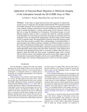
1746R. L. Nowack, W.-P. Chen, and T.-L. Tsengof about 25 km in width on each side of the array, outliningthe limit of lateral coverage of the data. When images fromall sources of illumination are stacked, average subsurfaceproperties of any potential small scale, lateral variationswithin this swath are imaged onto the profile (see furtherdiscussions on Fresnel zones in the following section).Gaussian-Beam Images from Individual AzimuthsIn this section, we present the individual GB migrationimages using stacked seismic data from each of the threeazimuths, southeast (SE), northeast (NE), and northwest(NW) of the array. Gaussian filters are chosen to minimizeside lobes from filtering when receiver functions are formed,and the results are shown for three different Gaussian widthsof Gw 0:90 (low frequency), 1.25 (mid frequency), and2.3 (high frequency), which correspond to reference frequencies of 0.24, 0.33, and 0.61 Hz where the Gaussian amplitudedecreases to 0.5. Comparisons among these images illustratethe multiscale nature of scattering beneath the array.Imaging algorithms require a background velocity model in order to determine the locations of the scatterers. For theHi-CLIMB data, we use a 2D or laterally varying backgroundmodel as described in Appendix B. We also tested laterallyhomogeneous models, and it turns out that the results of migration are not sensitive to specific details of the backgroundvelocity model. As noted before, we allow for the incidentwave to propagate through the 2D model at the appropriateincident angle and azimuth for each event group. In doing so,data from different stations along the profile are aligned bythe timing of the first P arrivals, and the timing of the incident wave field is correspondingly shifted.Figure 2 shows the GB migration results based on stackedreceiver functions from the 12 events located to the SE of thearray (Fig. 1a). In all images, reflectivity of scatterers is normalized to a range between 1 and 1, with positive andnegative values shown in blue and red colors, respectively.For reference, the locations of the IYS and BNS on the surfaceare also shown. The images cover the entire Lhasa terranebetween the IYS and the BNS and the southern and centralQiantang terrane to about 200 km north of the BNS.Between distances of 0 and 250 km, the low and midfrequency images at Gw of 0.9 and 1.25 (Fig. 2) show a coherent Moho scatterer at around 72 km in depth, with a shortsegment of disruption between distances of 120 and 150 km.Farther northward, the Moho is severely disrupted betweendistances from 250 to 350 km with enhanced lower crustalscattering. From 350 to 450 km reflectivity of the Moho isweak but then strengthens again between distances from 450to 550 km at a somewhat shallower depth (by about 10 km).As expected, more complicated Moho structures appearin higher frequency images. At distances less than 250 km,a deeper scattering feature can be seen between 100 and140 km in depth. Another deeper scattering structure can alsobe seen north of 300 km in distance and from 90 to 140 km inFigure 2.GB migration images formed by stacked receiverfunctions from 12 events to the SE of the Hi-CLIMB array shownin Figure 1a. The migration results are shown for three differentGaussian low-pass filters with Gaussian widths of Gw 0:90(low frequency), 1.25 (mid frequency), and 2.3 (high frequency).These values correspond to frequencies of 0.24, 0.33, and0.61 Hz, where the amplitude of each filter drops by a factor of2 of its peak value at 0 Hz.depth, possibly dipping to the north. But these deeper scattering features could be false images related to multiples.Figure 3 shows GB migration images for the NE stackedevents at three different frequency bands. Similar to resultsfrom the SE, the Moho reflectivity is strong in the southernportion of the profile, appearing at a depth of about 72 km.The Moho becomes complicated between distances 225 and300 km, and from 300 to 425 km reflectivity of the Moho isvery subdued. The Moho scattering then strengthens north ofabout 450 km in distance and is about 10 km shallower indepth then that under the southern end of the profile. In contrast to the SE migration results, any structure deeper than theMoho, between depths of 100 and 150 km, is inconspicuous.Finally, results from the NW events are shown inFigure 4. Note that both the quantity and quality of data inthis azimuth are not as favorable as those of the other twogroups. In Figure 4, Moho scattering is again strong in thesouthern portion of the profile, with some disruptions nearthe distance of 125 km but persists up to around 200 km,where it weakens. In contrast to the other two profiles, theMoho scattering is stronger between distances of 225 and upto the BNS but with some complicated midcrustal scattering.

Application of Gaussian-Beam Migration to Multiscale Imaging of Lithosphere beneath Hi-CLIMB ArrayFigure 3.GB migration images formed by stacked receiverfunctions from five events to the NE of the Hi-CLIMB array shownin Figure 1a. The layout is the same as that in Figure 2.1747(Nonetheless, notice that horizontal resolution along theprofile is high, on the order of 8 km or less as illustrated bytests with synthetic seismograms, Appendix A, Fig. A2).Furthermore, because a seismic deployment at the scaleof Hi-CLIMB is by necessity a temporary endeavor, thisconstraint limits the azimuthal coverage of data due to theintrinsic geometry and nonstationary nature of the Earth’sseismicity. As such, instead of appealing to exotic explanations that cannot be verified by existing data, we attribute anyapparent azimuthal variations in our results to slight deviations from a purely 2D geometry of geologic structures within the swath of conversion points around the array. As such,we perform final interpretations based on linear stacking ofimages from the three available azimuths (Fig. 5), bearing inmind the fact that the overall data quality and quantity arebest for the events from the SE and NE of the array.Before proceeding with the final interpretation, it is heuristic to recall that in addition to the great depth of penetrationfrom wave fields generated by large earthquakes, the broadband nature of signals from earthquakes is important. First,gradual changes in impedance are not particularly sensitiveto high-frequency waves, a common issue for earlier studiesin southern Tibet that rely on man-made sources of illumination (Hauck et al., 1998). Second, as spatial resolutionincreases with increasing frequency, so does the complexityof the resulting image. Comparison among the images fromReflectivity of the Moho weakens between distances of 370and 420 km and then strengthens again farther northward at ashallower depth. There appears to be some scattering belowthe Moho between depths of 100 and 180 km, but thesefeatures seem unstable, with considerable variations amongdifferent frequency bands.Stacked Gaussian-Beam Imagesand Geologic InterpretationsBecause successive collisions that built the Tibetan plateau are a result of northward convergence of fragments ofthe Gondwanaland toward stable Siberia (e.g., Tapponnieret al., 2001), the dominate trend of variation in geologicstructures is north–south. Nevertheless, lateral variations,albeit at a smaller scale, are abundant (e.g., Yin and Harrison,2000). Meanwhile, the geometry of the array is approximately 2D, so each group of events images somewhat different regions at depth, up to 25 km away from the projectedposition of the profile—a direct result of different incidenceangles (mainly in azimuth) of the incoming P waves frombelow (Fig. 1c). For the range of dominant frequencies usedhere, the radii of the Fresnel zone at a depth of 70 km areabout 14–23 km. These values are comparable to the halfwidth of the swath of conversion points straddling the array(Fig. 1c), calling for geological interpretations to rely uponstacked images from all three azimuthal groups of sources.Figure 4.GB migration images formed by stacked receiverfunctions from four events to the NW of the Hi-CLIMB array shownin Figure 1a. The layout is the same as that in Figure 2.

1748R. L. Nowack, W.-P. Chen, and T.-L. TsengFigure 5. Cross sections of the Tibetan lithosphere as imaged by GB migration of direct P-to-S wave conversions. The images are stackedfrom three basic images corresponding to sources from the SE, the NE, and the NW of the array (Figs. 2–4). The convention is that a scattererrepresenting an increase in impedance with depth results in a blue pixel centered on the position of the scatterer. (a)–(c) Facilitated by thebroadband nature of earthquake data, these images are formed at three different frequency bands. Prior to migration, signals are filtered withlow-pass Gaussian filters characterized by Gaussian widths of 0.90 (low frequency), 1.25 (mid frequency), and 2.30 (high frequency) Thelayout is the same as that in Figure 2. (d) Same image as in (b), with our interpretations of the Moho transition zone highlighted by blackcurves (dashed when uncertain).different frequencies allows geologic interpretations thatachieve a balance between high resolution and lateral continuity of feature. To this end, the image from the midfrequencyband works well. Note that we applied no smoothing to eitherthe pre- or postmigrated images.As expected, the strongest signal comes from the Moho inthe stacked images—a feature that is well imaged in all frequency bands (Fig. 5a–c). More important, characteristics ofthe Moho vary considerably over the profile. Near both endsof the profile, the Moho is a sharp, continuous interface, with anoticeable difference of about 10 km in crustal thickness. Thedifference in crustal thickness is important for understandinghow uniform, high elevation of central and Northern Tibet isbeing supported (see Tseng et al., 2009, for further discussions). Near a distance (x) of about 100 km (Fig. 5), thereappears to be a slight break in its continuity but otherwisethe Moho interface remains a well-defined, laterally continuous feature that shows only minor fluctuations for another100 km. However, between x 200 and 430 km, a wide zoneof disrupted Moho stands out. Even at low frequencies(Fig. 5a), it is apparent that the Moho is disrupted; insteadthe crust–mantle transition spans a large range of depthsfrom about 80 to 40 km. Figure 5d shows our interpretationof the current configuration of the Moho for the entire profileby highlighting scatterers with particularly strong impedancecontrast. Some of the details at depth are resolvable onlyat high frequencies. For instance, apparent imbricationsof the Moho near a distance of 250 km are best seen inFigure 5b,c.As a first approximation, we assume that the propertiesof the uppermost mantle are homogeneous and isotropic.Possible deviations from this approximation, such as fluctuations in the speed of mantle P waves, will affect the preciseinterpretation of the impedance contrast across the Moho,but positions of the prominent scatterers are not sensitiveto the details of the background seismic-wave speeds (seeAppendix B for further discussion).Traditionally, identification of a suture between twocolliding terranes is based on observations near the surface,characterized by a broad zone of allochthonous terranes,including fragments of exotic terranes, oceanic rocks, andaccretionary prisms from both sides of the main interveningocean. Consequently, the precise location of a complexsuture zone is often nonunique, because the answer dependson whether structural features (including ophiolites), patternsof isotopic ratios, or paleontological criteria are used

Application of Gaussian-Beam Migration to Multiscale Imaging of Lithosphere beneath Hi-CLIMB Array(Windley, 1995). On a lithospheric scale, the subsurface orgeophysical suture is the subsurface join between opposing,stable terranes (Marillier, 1989). In our case, it is straightforward to identify sharp, flat-lying portions of the Mohotoward the southern and northern ends of the cross sectionas stable mantle lithosphere of Lhasa and Qiangtang terranes,respectively (Fig. 5d).The fact that disrupted (therefore deformed) Moho islimited to the central portion of the profile points to considerable strength of the mantle lithosphere. If the mechanicalstrength of the entire lithosphere mainly resides in the crust(“crème brûlée”) (e.g., Jackson, 2002), deformation of theMoho should be as pervasive and widespread as the crustwhose top surface is undergoing significant pure shearthroughout the entire plateau (Meade, 2007; Thatcher, 2007).A strong lithospheric mantle is consistent with independentevidence from the occurrence of mantle earthquakes insouthern Tibet (Chen and Molnar, 1983; Chen and Yang,2004; de la Torre, 2007), favoring a bimodal distribution oflithospheric strength with maxima in the midcrust and nearthe Moho (“jelly sandwich”).Interestingly, the zone of disturbed Moho straddles theBNS, but there is no corresponding feature under the IYS.Such a difference suggests that the zone of disturbance nearthe BNS has been reworked during the most recent episode ofcollision and/or different processes that occurred during thetwo successive episodes of collision. An obvious piece ofsupporting evidence for the latter is the differences in the distribution of rocks and geologic structures near the surface.While the Lhasa terrane is largely covered by both eruptivevolcanism and large granitic plutons that mark the activecontinental margin prior to collision along the IYS (Yinand Harrison, 2000), the Qiangtang terrane is an anticlinorium with Mesozoic blueschist-bearing mélange and upperPaleozoic strata in the core (Kapp et al., 2005). Tapponnieret al. (2001) proposed that the BNS is associated with southward underthrust of the Qiangtang terrane (intracontinentalsubduction), while Kapp et al. (2005) emphasized contraction, with north-dipping imbricate thrust sheets near the surface and uniform crustal thickening at depth. Apparentimbrications of the Moho suggest that south-dipping thrustfaulting of the uppermost mantle could be involved (Fig. 5), aprocess currently active beneath the Himalayan deformationfront except that there the dip direction of the entire system istoward the north (Chen and Kao, 1996).The occurrence of more than one large impedance contrast in the zone of disrupted Moho could suggest that mafic,or even ultramafic, mantle materials have been incorporatedinto the thickened crust and some mantle materials nowreside in the mid- to lower crust (Fig. 5). This interpretationis supported by field evidence from mature collision zoneswhere erosion has exposed the deep anatomy of thickenedcrust. For instance, in the Norwegian Caledonide, a productof early Paleozoic collision between Baltica and Laurentia,van Roermund et al. (1998) and Scambelluri et al. (2008)reported detailed studies of the Ugelvik–Raudhaugene–1749Midsundvattnet peridotite bodies in the Western Gneiss region of Norway. This ultramafic body, originally emplaced atthe mid- to lower crustal level, is now exposed at the surfacewithin a highly metamorphosed continental crust where theMoho is currently at a depth of about 35 km (Artemieva andThybo, 2008). In Norway alone, there are numerous otherexamples of known ultramafic bodies in deformed continental crust (Brueckner and van Roermund, 2004).There has been a long-standing debate as to whetherdiffuse deformation, a characteristic of continental lithosphere, is best explained as interaction among discrete blocks(Tapponnier et al., 2001; Calais, et al., 2006) or deformationof a continuous medium (Houseman and England, 1993;Holt et al., 2000). Space-based geodetic measurements indicate that on a scale of 100 km or more, the surface of Tibetis currently under uniform strain (Meade, 2007; Thatcher,2007), with subsidiary contribution from motion across discrete faults. At depths of about 70 km beneath the thickenedcrust, our results show that there are stable blocks in the mantle portions of the lithosphere beneath both the Qiangtangand Lhasa terranes where the Moho is a laterally continuous,smooth-varying feature, visible via both high- and lowfrequency seismic waves (Fig. 5c). Between the two stableblocks is a wide zone of highly disrupted Moho, of comparable scale to that of the stable blocks ( 200 km). Thisobservation suggests that for the mantle lithosphere, themotion of discrete blocks and pervasive deformation overwide intervening zones are of about equal importance.ConclusionsWe applied GB migration of teleseismic P waves to image the lithosphere in Tibet using data from the linear arrayof the Hi-CLIMB experiment. We selected three-componentP-wave data from three groups of earthquakes, each within arestricted range of azimuth and distance, to form stacks ofradial receiver functions that we then used to image the lithosphere by GB migration. The broad bandwidth of the datafacilitates imaging at different frequency bands for eachazimuth, constraining multiscale scattering properties ofthe lithosphere. For each frequency band, images from eachgroup of illumination are then stacked to form a final GBimage for geologic interpretations.Overall, heterogeneities beneath a wide zone of about250 km in length near the BNS in the heartland of Tibet aremore pronounced than those under apparently stable terranesfarther to the south or the north. Specifically, P-to-S conversions across the Moho are generally strong and continuousunder much of the southern Lhasa terrane, corresponding to awell-defined Moho. A disrupted zone of

nous seismic data collected along the linear array of project Hi-CLIMB (Himalayan-Tibetan Continental Lithosphere during Mountain Building) (Nabelek et al., 2005) offer an excellent opportunity to address continental deformation on a lithospheric scale across the most prominent zone of active continental collision—the Himalayan-Tibetan .