Transcription
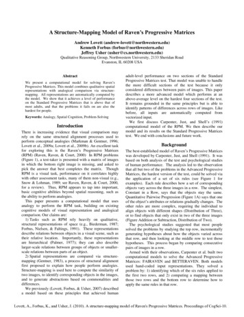
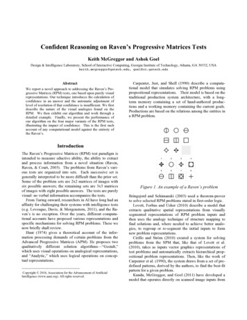
Confident Reasoning on Raven’s Progressive Matrices TestsKeith McGreggor and Ashok GoelDesign & Intelligence Laboratory, School of Interactive Computing, Georgia Institute of Technology, Atlanta, GA 30332, USAkeith.mcgreggor@gatech.edu, goel@cc.gatech.eduAbstractWe report a novel approach to addressing the Raven’s Progressive Matrices (RPM) tests, one based upon purely visualrepresentations. Our technique introduces the calculation ofconfidence in an answer and the automatic adjustment oflevel of resolution if that confidence is insufficient. We firstdescribe the nature of the visual analogies found on theRPM. We then exhibit our algorithm and work through adetailed example. Finally, we present the performance ofour algorithm on the four major variants of the RPM tests,illustrating the impact of confidence. This is the first suchaccount of any computational model against the entirety ofthe Raven’s.Carpenter, Just, and Shell (1990) describe a computational model that simulates solving RPM problems usingpropositional representations. Their model is based on thetraditional production system architecture, with a longterm memory containing a set of hand-authored productions and a working memory containing the current goals.Productions are based on the relations among the entities ina RPM problem.IntroductionThe Raven’s Progressive Matrices (RPM) test paradigm isintended to measure eductive ability, the ability to extractand process information from a novel situation (Raven,Raven, & Court, 2003). The problems from Raven’s various tests are organized into sets. Each successive set isgenerally interpreted to be more difficult than the prior set.Some of the problem sets are 2x2 matrices of images withsix possible answers; the remaining sets are 3x3 matricesof images with eight possible answers. The tests are purelyvisual: no verbal information accompanies the tests.From Turing onward, researchers in AI have long had anaffinity for challenging their systems with intelligence tests(e.g. Levesque, Davis, & Morgenstern, 2011), and the Raven’s is no exception. Over the years, different computational accounts have proposed various representations andspecific mechanisms for solving RPM problems. These wenow briefly shall review.Hunt (1974) gives a theoretical account of the information processing demands of certain problems from theAdvanced Progressive Matrices (APM). He proposes twoqualitatively different solution algorithms—“Gestalt,”which uses visual operations on analogical representations,and “Analytic,” which uses logical operations on conceptual representations.Copyright 2014, Association for the Advancement of ArtificialIntelligence (www.aaai.org). All rights reserved.Figure 1. An example of a Raven’s problemBringsjord and Schimanski (2003) used a theorem-proverto solve selected RPM problems stated in first-order logic.Lovett, Forbus and Usher (2010) describe a model thatextracts qualitative spatial representations from visuallysegmented representations of RPM problem inputs andthen uses the analogy technique of structure mapping tofind solutions and, where needed to achieve better analogies, to regroup or re-segment the initial inputs to formnew problem representations.Cirillo and Ström (2010) created a system for solvingproblems from the SPM that, like that of Lovett et al.(2010), takes as inputs vector graphics representations oftest problems and automatically extracts hierarchical propositional problem representations. Then, like the work ofCarpenter et al. (1990), the system draws from a set of predefined patterns, derived by the authors, to find the best-fitpattern for a given problem.Kunda, McGreggor, and Goel (2011) have developed amodel that operates directly on scanned image inputs from
the test. This model uses operations based on mental imagery (rotations, translations, image composition, etc.) toinduce image transformations between images in the problem matrix and then predicts an answer image based on thefinal induced transformation. McGreggor, Kunda, andGoel (2011) also report a model that employs fractal representations of the relationships between images.Finally, Rasmussen and Eliasmith (2011) used a spikingneuron model to induce rules for solving RPM problems.Input images from the test were hand-coded into vectors ofpropositional attribute-value pairs, and then the spikingneuron model was used to derive transformations amongthese vectors and abstract over them to induce a generalrule transformation for that particular problem.The variety of approaches to solving RPM problemssuggest that no one definitive account exists. Here, wedevelop a new method for addressing the RPM, based uponfractal representations. An important aspect of our methodis that a desired confidence with which the problem is to besolved may be used as a method for automatically tuningthe algorithm. In addition, we illustrate the application ofour model against all of the available test suites of RPMproblems, a first in the literature.example, this involves the calculation of a set of similarityvalues Θi for each answer Ai:Θi { S( H1, H(Ai) ), S( H2, H(Ai) ),S( V1, V(Ai) ), S( V2, V(Ai) ) }where H(Ai) and V(Ai) denote the relationship formedwhen the answer image Ai is included. S(X,Y) is theTversky featural similarity between two sets X and Y(Tversky, 1977):S(X,Y) f(X Y) / [ f(X Y) αf(X-Y) βf(Y-X) ]Fractal Representation of Visual RelationshipsWe chose to use fractal representations here for their consistency under re-representation (McGreggor, 2013), and inparticular for the mutual fractal representation, which expresses the relationship between sets of images.In Figure 3, we illustrate how to construct a mutual fractal representation of the relationship H1.Ravens and ConfidenceLet us illustrate our method for solving RPM problems.We shall use as an example the 3x3 matrix problem shownin Figure 1. The images and Java source code for this example may be found on our research group’s website.Figure 3. Mutual Fractal RepresentationsConfidence and AmbiguityFigure 2. Simultaneous relationshipsSimultaneous Relationships and ConstraintsIn any Raven’s problem there exist simultaneous horizontal and vertical relationships which must be maintained. InFigure 2, we illustrate these relationships using our example problem. As shown, relationships H1 and H2 constrainrelationship H, while relationships V1 and V2 constrainrelationship V. While there may be other possible relationships suggested by this problem, we have chosen to focuson these particular relationships for clarity.To solve a Raven’s problem, one must select the imagefrom the set of possible answers for which the similarity toeach of the problem’s relationships is maximal. For ourAn answer to a Raven’s problem may be found by choosing the one with the maximal featural similarity. But howconfident is that answer? Given the variety of answerchoices, even though an answer may be selected based onmaximal similarity, how may that choice be contrastedwith its peers as the designated answer?We claim that the most probable answer would in asense “stand apart” from the rest of the choices, and thatdistinction may be interpreted as a metric of confidence.Assuming a normal distribution, we may calculate a confidence interval based upon the standard deviation, and scoreeach of these values along such a confidence scale. Thus,the problem of selecting the answer for a Raven’s problemis transformed into a problem of distinguishing which ofthe possible choices is a statistical outlier.
The Confident Ravens AlgorithmTo address Raven’s problems, we developed the ConfidentRavens algorithm. We present it here in pseudo-codeform, in two parts: the preparatory stage and the executionstage.Confident Ravens, Preparatory StageIn the first stage of our Confident Ravens Algorithm, animage containing the entire problem is first segmented intoits component images (the matrix of images, and the possible answers). Next, based upon the complexity of the matrix, the set of relationships to be evaluated is established.Then, a range of abstraction levels is determined.Throughout, we use MutualFractal() to indicate the mutualfractal representation of the input images (McGreggor &Goel, 2012).In the present implementation, the abstraction levels aredetermined to be a partitioning of the given images intogridded sections at a prescribed size and regularity.Confident Ravens, Execution StageThe algorithm concludes by calculating similarity valuesfor each of the possible answer choices. It uses the deviation of these values from their mean to determine the confidence in the answers at each level.Given M, C, R, A, and η as determined in the preparatorystage, determine an answer and its confidence.Let Ε be a real number which represents the number ofstandard deviations beyond which a value’s answer may bejudged as “confident”Let S(X,Y) be the Tversky similarity metric for sets X and YEXECUTIONGiven an image P containing a Raven’s problem, prepare todetermine an answer with confidence.PROBLEM SEGMENTATIONBy examination, divide P into two images, one containing thematrix and the other containing the possible answers. Further divide the matrix image into an ordered set of either 3 or8 matrix element images, for 2x2 or 3x3 matrices respectively. Likewise, divide the answer image into an ordered set ofits constituent individual answer choices.Let M { m1, m2, . } be the set of matrix element images.Let C { c1, c2, c3, . } be the set of answer choices.Let η be an integer denoting the order of the matrix image(either 2 or 3, for 2x2 or 3x3 matrices respectively).RELATIONSHIP DESIGNATIONSLet R be a set of relationships, determined by the value of ηas follows:If η 2:R { H1, V1 } whereH1 MutualFractal( m1, m2 )V1 MutualFractal( m1, m3 )Else: (because η 3)R { H1, H2, V1, V2 } whereH1 MutualFractal( m1, m2 , m3 )H2 MutualFractal( m4, m5 , m6 )V1 MutualFractal( m1, m4 , m7 )V2 MutualFractal( m2, m5 , m8 )ABSTRACTION LEVEL PREPARATIONLet d be the largest dimension for any image in M C.Let A : { a1, a2, . } represent an ordered range of abstraction values wherea1 d, and ai ½ ai-1 i, 2 i floor( log2 d ) and ai 2The values within A constitute the grid values to be usedwhen partitioning the problem’s images.Algorithm 1. Confident Ravens Preparatory StageFor each abstraction a A: Re-represent each representation r R according toabstraction a S For each answer image c C : If η 2:H MutualFractal( m3, c )V MutualFractal( m2, c )Θ { S( H 1, H ), S( V1, V ) } Else: (because η 3)H MutualFractal( m7, m8, c )V MutualFractal( m3, m6, c )Θ { S( H 1, H ), S( H2, H ),S( V1, V ), S( V2, V ) } Calculate a single similarity metric from vector Θ:t Σ θ2 θ ΘS S { t } Set µ mean ( S ) Set σµ stdev ( S ) / n Set D { D1, D2, D3, D4, . Dn }where Di (Si-µ) / σµ Generate the set Z { Zi . } Zi D and Zi E If Z 1, return the answer image ci C which corresponds to Zi otherwise there exists ambiguity, and further refinement must occur.If no answer has been returned, then no answer may be givenunambiguously.Algorithm 2. Confident Ravens Execution StageThus, for each level of abstraction, the relationships implied by the kind of Raven’s problem (2x2 or 3x3) are rerepresented into that partitioning. Then, for each of thecandidate images, a potentially analogous relationship isdetermined for each of the existing relationships and a similarity value calculated. The vector of similarity values isreduced via a simple Euclidean distance formula to a singlesimilarity. The balance of the algorithm, using the deviation from the mean of these similarities, continues through
a variety of levels of abstraction, looking for an unambiguous answer that meets the specified confidence constraint.The Example, SolvedTable 1 shows the results of running the Confident Ravensalgorithm on the example problem, starting at an originalgridded partitioning of 200x200 pixels (the maximal pixeldimension of the images), and then refining the partitioning down to a grid of 6x6 pixels, using a subdivision byhalf scheme, yielding 6 levels of abstraction.Let us suppose that a confidence level of 95% is desired.The table gives the mean (µ), standard deviation (σµ), andnumber of features (f) for each level of abstraction (grid).The deviation and confidence for each candidate answerare given for each level of abstraction as well.imagedeviations & 898.06%1.92294.54%gr 42436968Table 1. Image Deviations and ConfidencesYellow indicates ambiguous results, red indicates thatthe result is unambiguousThe deviations presented in table 1 appear to suggest that ifone starts at the very coarsest level of abstraction, the answer is apparent (image choice 3). Indeed, the confidencein that answer never dips below 99.66%.We see evidence that operating with either too sparse adata set (at the coarsest) or with too homogeneous a dataset (at the finest) may be problematic. The coarsest abstraction (200 pixel grid size) offers 378 features, whereasthe finest abstraction (6 pixel grid size) offers more than400,000 features for consideration.The data in the table suggests the possibility of automatically detecting these boundary situations. We note thatthe average similarity measurement at the coarsest abstraction is 0.589, but then falls, at the next level of abstraction,to 0.310, only to thereafter generally increase. This constitutes further evidence for an emergent boundary for themaximum coarse abstraction.We surmise that ambiguity exists for ranges of abstraction, only to vanish at some appropriate levels of abstraction, and then reemerges once those levels are surpassed.The example here offers evidence of such behavior, wherethere exists ambiguity at grid sizes 100, 50, 25, and 12,then the ambiguity vanishes for grid size 6. Though weomit the values in Table 1 for clarity of presentation, ourcalculations show that ambiguity reemerges for grid size 3.This suggests that there are discriminatory features withinthe images exist only at certain levels of abstraction.ResultsWe have tested the Confident Ravens algorithm against thefour primary variants of the RPM: the 60 problems of theStandard Progressive Matrices (SPM) test, the 48 problemsof the Advanced Progressive Matrices (APM) test, the 36problems of the Coloured Progressive Matrices (CPM) test,and the 60 problems of the SPM Plus test. Insofar as weknow, this research represents the first published computational account of any model against the entire suite of theRaven Progressive Matrices.To create inputs for the algorithm, each page from thevarious Raven test booklets were scanned, and the resulting greyscale images were rotated to roughly correct forpage alignment issues. Then, the images were sliced up tocreate separate image files for each entry in the problemmatrix and for each answer choice. These separate imageswere the inputs to the technique for each problem. No further image processing or cleanup was performed, despitethe presence of numerous pixel-level artifacts introducedby the scanning and minor inter-problem image alignmentissues. Additionally, each problem was solved independently: no information was carried over from problemto problem, nor from test variant to test variant.The code used to conduct these tests was precisely thesame code as used in the presented example, and is availa-
ble for download from our lab website. The Raven testimages as scanned, however, are copyrighted and thus arenot available for download.Performance on the APM test: 43 of 48On the Raven’s Advanced Progressive Matrices (APM)test, the Confident Ravens algorithm detected the correctanswer at a 95% or higher level of confidence on 43 of the48 problems. The number of problems with detected correct answers per set were 11 for set A, and 32 for set B. Ofthe 43 problems where the correct answers detected, 27problems were answered ambiguously.Abstractions, Metrics, and CalculationsThe images associated with each problem, in general, had amaximum pixel dimension of between 150 and 250 pixels.We chose a partitioning scheme which started at the maximum dimension, then descended in steps of 10, until itreached a minimum size of no smaller than 4 pixels, yielding 14 to 22 levels of abstraction for each problem.At each level of abstraction, we calculated the similarityvalue for each possible answer, as proscribed by the Confident Ravens algorithm. For those calculations, we used theTversky contrast ratio formula (1977), and set α to 1.0 andβ equal to 0.0, conforming to values used in the coincidence model by Bush and Mosteller (1953), yielding anasymmetric similarity metric preferential to the problemmatrix’s relationships. From those values, we calculatedthe mean and standard deviation, and then calculated thedeviation and confidence for each answer. We made noteof which answers provided a confidence above our chosenlevel, and whether for each abstraction level the answerwas unambiguous or ambiguous, and if ambiguous, in whatmanner.As we were exploring the advent and disappearance ofambiguity and the effect of confidence, we chose to allowthe algorithm to run fully at all available levels of abstraction, rather than halting when an unambiguous answer wasdetermined.Performance on the CPM test: 35 of 36On the Raven’s Coloured Progressive Matrices (CPM) test,the Confident Ravens algorithm detected the correct answer at a 95% or higher level of confidence on 35 of the 36problems. The number of problems with detected correctanswers per set were 12 for set A, 12 for set AB, and 11 forset B. Of the 35 problems where the correct answers detected, 5 problems were answered ambiguously.Performance on the SPM Plus test: 58 of 60On the Raven’s SPM Plus test, the Confident Ravens algorithm detected the correct answer at a 95% or higher levelof confidence on 58 of the 60 problems. The number ofproblems with detected correct answers per set were 12 forset A, 11 for set B, 12 for set C, 12 for set D, and 11 for setE. Of the 58 problems where the correct answers detected,23 problems were answered ambiguously.Confidence and Ambiguity, RevisitedWe explored a range of confidence values for each testsuite of problems, and illustrate these findings in Table 2.Note that as confidence increases from 95% to 99.99%,the test scores decrease, but so too does the ambiguity.Analogously, as the confidence is relaxed from 95% downto 60%, test scores increase, but so too does ambiguity. Byinspection, we note that there is a marked shift in the rateat which test scores and ambiguity change between 99.9%and 95%, suggesting that 95% confidence may be a reasonable choice.Performance on the SPM test: 54 of 60On the Raven’s Standard Progressive Matrices (SPM) test,the Confident Ravens algorithm detected the correct answer at a 95% or higher level of confidence on 54 of the 60problems. The number of problems with detected correctanswers per set were 12 for set A, 10 for set B, 12 for setC, 8 for set D, and 12 for set E. Of the 54 problems wherethe correct answers detected, 22 problems were answeredambiguously.confidencethr esholdSPM 60APM 48CPM 36SPMPlus 60cor r ectambiguouscor r ectambiguouscor r ectambiguouscor r 280%57364538369593760%5842474536146045Table 2. The Effect of Confidence on Score and Ambiguity
Our findings indicate that at 95% confidence, thoseproblems which are answered correctly but ambiguouslyare vacillating almost in every case between two choices(out of an original 6 or 8 possible answers for the problem). This narrowing of choices suggests to us that ambiguity resolution might entail a closer examination of justthose specific selections, via re-representation as affordedby the fractal representation, a change of representationalframework, or a change of algorithm altogether.Comparison to other computational modelsAs we noted in the introduction, there are other computational models which have been used on some or all problems of certain tests. However, all other computationalaccounts report scores when choosing a single answer perproblem, and do not report at all the confidence with whichtheir algorithms chose those answers. As such, our reportedtotals must be considered as a potential high score for Confident Ravens if the issues of ambiguity were to be sufficiently addressed.Also as we noted earlier, this paper presents the firstcomputational account of a model running against all fourvariants of the RPM. Other accounts generally reportscores on the SPM or the APM, and no other account existsfor scores on the SPM Plus.Carpenter et al. (1990) report results of running two versions of their algorithm (FairRaven and BetterRaven)against a subset of the APM problems (34 of the 48 total).The subset of problems chosen by Carpenter et al. reflectthose whose rules and representations were deemed as inferable by their production rule based system. They reportthat FairRaven achieves a score of 23 out of the 34, whileBetterRaven achieves a score of 32 out of the 34.Lovett et al (2007, 2010) report results from their computational model’s approach to the Raven’s SPM test. Ineach account, only a portion of the test was attempted, butLovett et al project an overall score based on the performance of the attempted sections. The latest published account by Lovett et al (2010) reports a score of 44 out of 48attempted problems from sets B through E of the SPM test,but does not offer a breakdown of this score by problemset. Lovett et al. (2010) project a score of 56 for the entiretest, based on human normative data indicating a probablescore of 12 on set A given their model’s performance onthe attempted sets.Cirillo and Ström (2010) report that their system wastested against Sets C through E of the SPM and solved 8,10, and 10 problems, respectively, for a score of 28 out ofthe 36 problems attempted. Though unattempted, theypredict that their system would score 19 on the APM (aprediction of 7 on set A, and 12 on set B).Kunda et al. (2013) reports the results of running theirASTI algorithms against all of the problems on both theSPM and the APM tests, with a detailed breakdown ofscoring per test. They report a score of 35 for the SPMtest, and a score of 21 on the APM test. In her dissertation,Kunda (2013) reports a score of 50 for the SPM, 18 for theAPM, and 35 on the CPM.McGreggor et al. (2011) contains an account of runninga preliminary version of their algorithm using fractal representations against all problems on the SPM. They report ascore of 32 on the SPM, 11 on set A, 7 on set B, 5 on set C,7 on set D, and 2 on set E. They report that these resultswere consistent with human test taker norms. Kunda et al.(2012) offers a summation of the fractal algorithm as applied to the APM, with a score of 38, 12 on set A, and 26on set B.The work we present here represents a substantial theoretical extension as well as a significant performance improvement upon these earlier fractal results.ConclusionIn this paper, we have presented a comprehensive accountof our efforts to address the entire Raven’s ProgressiveMatrices tests using purely visual representations, the firstsuch account in the literature. We developed the ConfidentRavens algorithm, a computational model which uses features derived from fractal representations to calculateTversky similarities between relationships in the test problem matrices and candidate answers, and which uses levelsof abstraction, through re-representing the visual representation at differing resolutions, to determine overall confidence in the selection of an answer. Finally, we presenteda comparison of the results of running the Confident Ravens algorithm to all available published accounts, andshowed that the Confident Ravens algorithm’s performance at detecting the correct answer is on par with thoseaccounts.The claim that we present throughout these results, however, is that a computational model may provide both ananswer as well as a characterization of the confidence withwhich the answer is given. Moreover, we have shown thatinsufficient confidence in a selected answer may be usedby that computational model to force a reconsideration of aproblem, through re-representation, representational shift,or algorithm change. Thus, we suggest that confidence ishereby well-established as a motivating factor for reasoning, and as a potential drive for an intelligent agent.AcknowledgmentsThis work has benefited from many discussions with ourcolleague Maithilee Kunda and the members of the Designand Intelligence Lab at Georgia Institute of Technology.We thank the US National Science Foundation for its support of this work through IIS Grant #1116541, entitled“Addressing visual analogy problems on the Raven’s intelligence test.”
ReferencesBarnsley, M., and Hurd, L. 1992. Fractal Image Compression.Boston, MA: A.K. Peters.Bringsjord, S., and Schimanski, B. 2003. What is artificial intelligence? Psychometric AI as an answer. International Joint Conference on Artificial Intelligence, 18: 887–893.Bush, R.R., and Mosteller, F. 1953. A Stochastic Model withApplications to Learning. The Annals of Mathematical Statistics,24(4): 559-585.Carpenter, P., Just, M., and Shell, P. 1990. What one intelligencetest measures: a theoretical account of the processing in the Raven Progressive Matrices Test. Psychological Review, 97(3): 404431.Cirillo, S., and Ström, V. 2010. An anthropomorphic solver forRaven’s Progressive Matrices (No. 2010:096). Goteborg, Sweden: Chalmers University of Technology.Haugeland, J. ed. 1981. Mind Design: Philosophy, Psychologyand Artificial Intelligence. MIT Press.Hofstadter, D., and Fluid Analogies Research Group. eds. 1995.Fluid concepts & creative analogies: Computer models of thefundamental mechanisms of thought. New York: Basic Books.Hunt, E. 1974. Quote the raven? Nevermore! In L. W. Gregg ed.,Knowledge and Cognition (pp. 129–158). Hillsdale, NJ: Erlbaum.Kunda, M. 2013. Visual Problem Solving in Autism, Psychometrics, and AI: The Case of the Raven's Progressive MatricesIntelligence Test. Doctoral dissertation, Georgia Institute ofTechnology.Kunda, M., McGreggor, K. and Goel, A. 2011. Two Visual Strategies for Solving the Raven’s Progressive Matrices IntelligenceTest. Proceedings of the 25th AAAI Conference on Artificial Intelligence.Kunda, M., McGreggor, K. and Goel, A. 2012. Reasoning on theRaven’s Advanced Progressive Matrices Test with Iconic VisualRepresentations. Proceedings of the 34th Annual Meeting of theCognitive Science Society, Sapporo, Japan.Kunda, M., McGreggor, K., & Goel, A. K. 2013. A computational model for solving problems from the Raven's Progressive Matrices intelligence test using iconic visual representations. Cognitive Systems Research, 22-23, pp. 47-66.Levesque, H. J., Davis, E., & Morgenstern, L. 2011. The Winograd Schema Challenge. In AAAI Spring Symposium: LogicalFormalizations of Commonsense Reasoning.Lovett, A. Forbus, K., and Usher, J. 2007. Analogy with qualitative spatial representations can simulate solving Raven's Progressive Matrices. Proceedings of the 29th Annual Conference of theCognitive Science Society.Lovett, A., Forbus, K., and Usher, J. 2010. A structure-mappingmodel of Raven’s Progressive Matrices. Proceedings of the 32ndAnnual Conference of the Cognitive Science Society.Mandelbrot, B. 1982. The fractal geometry of nature. San Francisco: W.H. Freeman.McGreggor, K. (2013). Fractal Reasoning. Doctoral dissertation, Georgia Institute of Technology.McGreggor, K., Kunda, M., & Goel, A. K. (2011). Fractal Analogies: Preliminary Results from the Raven's Test of Intelligence. InProceedings of the Second International Conference on Computational Creativity (ICCC), Mexico City. pp. 69-71.McGreggor, K., & Goel, A. 2011. Finding the odd one out: afractal analogical approach. Proceedings of the 8th ACM conference on Creativity and cognition (pp. 289-298). ACM.McGreggor, K., and Goel, A. 2012. Fractal analogies for generalintelligence. Artificial General Intelligence. Springer Berlin Heidelberg, 177-188.Raven, J., Raven, J. C., and Court, J. H. 2003. Manual forRaven's Progressive Matrices and Vocabulary Scales. San Antonio, TX: Harcourt Assessment.Rasmussen, D., and Eliasmith, C. 2011. A neural model of rulegeneration in inductive reasoning. Topics in Cognitive Science,3(1), 140-153.Tversky, A. 1977. Features of similarity. Psychological Review,84(4), 327-352.
the Raven's. Introduction The Raven's Progressive Matrices (RPM) test paradigm is intended to measure eductive ability, the ability to extract and process information from a novel situation (Raven, Raven, & Court, 2003). The problems from Raven's vari-ous tests are organized into sets. Each successive set is