Transcription
R2-B2: Recursive Reasoning-Based Bayesian Optimization forNo-Regret Learning in GamesZhongxiang Dai 1 Yizhou Chen 1 Bryan Kian Hsiang Low 1 Patrick Jaillet 2 Teck-Hua Ho 3AbstractThis paper presents a recursive reasoning formalism of Bayesian optimization (BO) to modelthe reasoning process in the interactions betweenboundedly rational, self-interested agents withunknown, complex, and costly-to-evaluate payoff functions in repeated games, which we callRecursive Reasoning-Based BO (R2-B2). OurR2-B2 algorithm is general in that it does not constrain the relationship among the payoff functionsof different agents and can thus be applied to various types of games such as constant-sum, generalsum, and common-payoff games. We prove thatby reasoning at level 2 or more and at one levelhigher than the other agents, our R2-B2 agentcan achieve faster asymptotic convergence to noregret than that without utilizing recursive reasoning. We also propose a computationally cheapervariant of R2-B2 called R2-B2-Lite at the expenseof a weaker convergence guarantee. The performance and generality of our R2-B2 algorithm areempirically demonstrated using synthetic games,adversarial machine learning, and multi-agent reinforcement learning.1. IntroductionSeveral fundamental machine learning tasks in the realworld involve intricate interactions between boundedly rational1 , self-interested agents that can be modeled as a formof repeated games with unknown, complex, and costly-toevaluate payoff functions for the agents. For example, in1Department of Computer Science, National University of Singapore, Republic of Singapore 2 Department of Electrical Engineering and Computer Science, Massachusetts Institute of Technology,USA 3 NUS Business School, National University of Singapore,Republic of Singapore. Correspondence to: Bryan Kian HsiangLow lowkh@comp.nus.edu.sg .Proceedings of the 37 th International Conference on MachineLearning, Online, PMLR 119, 2020. Copyright 2020 by the author(s).1Boundedly rational agents are subject to limited cognition andtime in making decisions (Gigerenzer & Selten, 2002).adversarial machine learning (ML), the interactions betweenthe defender D and the attacker A of an ML model can bemodeled as a repeated game in which the payoffs to D andA are the performance of the ML model (e.g., validation accuracy) and its negation, respectively. Specifically, given afully trained image classification model (say, provided as anonline service), A attempts to fool the ML model into misclassification through repeated queries of the model usingperturbed input images. On the other hand, for each queriedimage that is perturbed by A, D tries to ensure the correctness of its classification by transforming the perturbedimage before feeding it into the ML model. As anotherexample, multi-agent reinforcement learning (MARL) inan episodic environment can also be modeled as a repeatedgame in which the payoff to each agent is its return fromthe execution of all the agents’ selected policies.Solving such a form of repeated games in a cost-efficientmanner is challenging since the payoff functions of theagents are unknown, complex (e.g., possibly noisy, nonconvex, and/or with no closed-form expression/derivative),and costly to evaluate. Fortunately, the payoffs corresponding to different actions of each agent tend to be correlated.For example, in adversarial ML, the correlated perturbationsperformed by the attacker A (and correlated transformationsexecuted by the defender D) are likely to induce similareffects on the performance of the ML model. Such a correlation can be leveraged to predict the payoff associatedwith any action of an agent using a surrogate model suchas the rich class of Bayesian nonparametric Gaussian process (GP) models (Rasmussen & Williams, 2006) which isexpressive enough to represent a predictive belief of the unknown, complex payoff function over the action space of theagent. Then, in each iteration, the agent can select an actionfor evaluating its unknown payoff function that trades off between sampling at or near to a likely maximum payoff basedon the current GP belief (exploitation) vs. improving theGP belief (exploration) until its cost/sampling budget is expended. To do this, the agent can use a sequential black-boxoptimizer such as the celebrated Bayesian optimization (BO)algorithm (Shahriari et al., 2016) based on the GP-upperconfidence bound (GP-UCB) acquisition function (Srinivaset al., 2010), which guarantees asymptotic no-regret performance and is sample-efficient in practice. How then can
R2-B2: Recursive Reasoning-Based Bayesian Optimization for No-Regret Learning in Gameswe design a BO algorithm to account for its interactionswith boundedly rational1 , self-interested agents and stillguarantee the trademark asymptotic no-regret performance?Inspired by the cognitive hierarchy model ofgames (Camerer et al., 2004), we adopt a recursivereasoning formalism (i.e., typical among humans) to modelthe reasoning process in the interactions between boundedlyrational1 , self-interested agents. It comprises k levels ofreasoning which represents the cognitive limit of the agent.At level k 0 of reasoning, the agent randomizes its choiceof actions. At a higher level k 1 of reasoning, the agentselects its best response to the actions of the other agentswho are reasoning at lower levels 0, 1, . . . , k 1.This paper presents the first recursive reasoning formalismof BO to model the reasoning process in the interactionsbetween boundedly rational1 , self-interested agents with unknown, complex, and costly-to-evaluate payoff functions inrepeated games, which we call Recursive Reasoning-BasedBO (R2-B2) (Section 3). R2-B2 provides these agents withprincipled strategies for performing effectively in this typeof game. In this paper, we consider repeated games withsimultaneous moves and perfect monitoring2 . Our R2-B2algorithm is general in that it does not constrain the relationship among the payoff functions of different agents and canthus be applied to various types of games such as constantsum games (e.g., adversarial ML in which the attacker A anddefender D have opposing objectives), general-sum games(e.g., MARL where all agents have possibly different yet notnecessarily conflicting goals), and common-payoff games(i.e., all agents have identical payoff functions). We provethat by reasoning at level k 2 and one level higher than theother agents, our R2-B2 agent can achieve faster asymptoticconvergence to no regret than that without utilizing recursive reasoning (Section 3.1.3). We also propose a computationally cheaper variant of R2-B2 called R2-B2-Lite at theexpense of a weaker convergence guarantee (Section 3.2).The performance and generality of R2-B2 are demonstratedthrough extensive experiments using synthetic games, adversarial ML, and MARL (Section 4). Interestingly, weempirically show that by reasoning at a higher level, ourR2-B2 defender is able to effectively defend against theattacks from the state-of-the-art black-box adversarial attackers (Section 4.2.2), which can be of independent interestto the adversarial ML community.2. Background and Problem FormulationFor simplicity, we will mostly focus on repeated games between two agents, but have extended our R2-B2 algorithmto games involving more than two agents, as detailed inAppendix B. To ease exposition, throughout this paper, wewill use adversarial ML as the running example and thusrefer to the two agents as the attacker A and the defender D.For example, the input action space X1 Rd1 of A can bea set of allowed perturbations of a test image while the inputaction space X2 Rd2 of D can represent a set of feasibletransformations of the perturbed test image. We considerboth input domains X1 and X2 to be discrete for simplicity;generalization of our theoretical results in Section 3 to continuous, compact domains can be easily achieved through asuitable discretization of the domains (Srinivas et al., 2010).When the ML model is an image classification model, thepayoff function f1 : X1 X2 R of A, which takes in itsperturbation x1 X1 and D’s transformation x2 X2 asinputs, can be the maximum predictive probability amongall incorrect classes for a test image since A intends to causemisclassification. Since A and D have opposing objectives(i.e., D intends to prevent misclassification), the payoff function f2 : X1 X2 R of D can be the negation of that ofA, thus resulting in a constant-sum game between A and D.In each iteration t 1, . . . , T of the repeated game withsimultaneous moves and perfect monitoring23 , A and Dselect their respective input actions x1,t and x2,t simultaneously using our R2-B2 algorithm (Section 3) for evaluatingtheir payoff functions f1 and f2 . Then, A and D receive therespective noisy observed payoffs y1,t , f1 (x1,t , x2,t ) 1and y2,t , f2 (x1,t , x2,t ) 2 with i.i.d. Gaussian noises i N (0, σi2 ) and noise variances σi2 for i 1, 2.A common practice in game theory is to measure the performance of A via its (external) regret (Nisan et al., 2007):R1,T ,PT t 1 [f1 (x1 , x2,t ) f1 (x1,t , x2,t )](1)PTwhere x 1 , arg maxx1 X1 t 1 f1 (x1 , x2,t ). The external regret R2,T of D is defined in a similar manner. Analgorithm is said to achieve asymptotic no regret if R1,Tgrows sub-linearly in T , i.e., limT R1,T /T 0. Intuitively, by following a no-regret algorithm, A is guaranteedto eventually find its optimal input action x 1 in hindsight,regardless of D’s sequence of input actions.2In each iteration of a repeated game with (a) simultaneous moves and (b) perfect monitoring, every agent, respectively,(a) chooses its action simultaneously without knowing the otheragents’ selected actions, and (b) has access to the entire historyof game plays, which includes all actions selected and payoffsobserved by every agent in the previous iterations.To guarantee no regret (Section 3), A represents a predictivebelief of its unknown, complex payoff function f1 using therich class of Gaussian process (GP) models by modelingf1 as a sample of a GP (Rasmussen & Williams, 2006). Ddoes likewise with its unknown f2 . Interested readers are3Note that in some tasks such as adversarial ML, the requirement of perfect monitoring can be relaxed considerably. Refer toSection 4.2.2 for more details.
R2-B2: Recursive Reasoning-Based Bayesian Optimization for No-Regret Learning in Gamesreferred to Appendix A.1 for a detailed background on GP.In particular, A uses the GP predictive/posterior belief of f1to compute a probabilistic upper bound of f1 called the GPupper confidence bound (GP-UCB) (Srinivas et al., 2010)at any joint input actions (x1 , x2 ), which will be exploitedby our R2-B2 algorithm (Section 3): (2) σt 1 (x1 , x2 ) 1/2α1,t (x1 , x2 ) , µt 1 (x1 , x2 ) βtAlgorithm 1 R2-B2 for attacker A’s level-k reasoning1: for t 1, 2, . . . , T doSelect input action x1,t using its level-k strategy2:(while defender D selects input action x2,t )3:Observe noisy payoff y1,t f1 (x1,t , x2,t ) 14:Update GP posterior belief using h(x1,t , x2,t ), y1,t ibest-responds3.1. Recursive Reasoning Formalism of BOOur recursive reasoning formalism of BO follows a similarprinciple as the cognitive hierarchy model (Camerer et al.,2004): At level k 0 of reasoning, A adopts some randomized/mixed strategy of selecting its action. At level k 1of reasoning, A best-responds to the strategy of D who isreasoning at a lower level. Let xk1,t denote the input actionx1,t selected by A’s strategy from reasoning at level k initeration t. Depending on the (a) degree of knowledge aboutD and (b) available computational resource, A can chooseone of the following three types of strategies of selecting itsaction with varying levels of reasoning, as shown in Fig. 1:Level-k 0 Strategy. Without knowledge of D’s level ofreasoning nor its level-0 strategy, A by default can reason at0level 0 and play a mixed strategy P1,tof selecting its action00by sampling x1,t from the probability distribution P1,toverits input action space X1 , as discussed in Section 3.1.1.Mixed StrategyAttackerMixed Strategy Algorithm 1 describes the R2-B2 algorithm from the perspective of attacker A which we will adopt in this section.Our R2-B2 algorithm for defender D can be derived analogously. We will now discuss the recursive reasoning formalism of BO for A’s action selection in step 2 of Algorithm 1.Mixed Strategy 3. Recursive Reasoning-Based BayesianOptimization (R2-B2)best-responds 2for iteration t where µt 1 (x1 , x2 ) and σt 1(x1 , x2 ) denote,respectively, the GP posterior mean and variance at (x1 , x2 )(Appendix A.1) conditioned on the history of game playsup till iteration t 1 that includes A’s observed payoffs andthe actions selected by both agents in iterations 1, . . . , t 1.The GP-UCB acquisition function α2,t for D is defined likewise. Supposing A knows the input action x2,t selected byD and chooses an input action x1 to maximize the GP-UCBacquisition function α1,t (2), its choice involves trading offbetween sampling close to an expected maximum payoff(i.e., with large GP posterior mean) given the current GPbelief of f1 (exploitation) vs. that of high predictive uncertainty (i.e., with large GP posterior variance) to improve theGP belief of f1 (exploration) where the parameter βt is set totrade off between exploitation vs. exploration for boundingits external regret (1), as specified later in Theorem 1.Defender(a) Level 0AttackerDefender(b) Level 1AttackerDefender(c) Level 2Figure 1. Illustration of attacker A’s strategies of selecting its inputaction from reasoning at levels k 0, 1, and 2.Level-k 1 Strategy. If A thinks that D reasons at level00 and has knowledge of D’s level-0 mixed strategy P2,t,then A can reason at level 1 and play a pure strategy thatbest-responds to the level-0 strategy of D, as explained inSection 3.1.2. Such a level-1 reasoning of A is generalsince it caters to any level-0 strategy of D and hence doesnot require D to perform recursive reasoning.Level-k 2 Strategy. If A thinks that D reasons at levelk 1, then A can reason at level k and play a pure strategythat best-responds to D’s level-(k 1) action, as detailed inSection 3.1.3. Different from the level-1 reasoning of A, itslevel-k reasoning assumes that D’s level-(k 1) action isderived using the same recursive reasoning process.3.1.1. L EVEL -k 0 S TRATEGYLevel 0 is a conservative, default choice for A since it doesnot require any knowledge about D’s strategy of selectingits input action and is computationally lightweight. At level00, A plays a mixed strategy P1,tby sampling x01,t from the0probability distribution P1,tover its input action space X1 :0x01,t P1,t. A mixed/randomized strategy (instead of apure/deterministic strategy) is considered because withoutknowledge of D’s strategy, A has to treat D as a black-boxadversary. This setting corresponds to that of an adversarialbandit problem in which any deterministic strategy suffers from linear worst-case regret (Lattimore & Szepesvári,2020) and randomization alleviates this issue. Such a randomized design of our level-0 strategies is consistent withthat of the cognitive hierarchy model in which a level-0thinker does not make any assumption about the other agentand selects its action via a probability distribution withoutusing strategic thinking (Camerer et al., 2004). We will now
R2-B2: Recursive Reasoning-Based Bayesian Optimization for No-Regret Learning in Gamespresent a few reasonable choices of level-0 mixed strategies.However, in both theory (Theorems 2, 3 and 4) and practice,any strategy of action selection (including existing methods(Section 4.2.2)) can be considered as a level-0 strategy.of actions selected by D but not its observed payoffs, whichis the same as that needed by GP-MW. Our first main result(see its proof in Appendix C) bounds the expected regret ofA when using R2-B2 for level-1 reasoning:In the simplest setting where A has no knowledge of D’sstrategy, a natural choice for its level-0 mixed strategy israndom search. That is, A samples its action from a uniform distribution over X1 . An alternative choice is to usethe EXP3 algorithm for the adversarial linear bandit problem, which requires the GP to be transformed via a random features approximation (Rahimi & Recht, 2007) intolinear regression with random features as inputs. Sincethepregret of EXP3 algorithm is bounded from above byO( d01 T log X1 ) (Lattimore & Szepesvári, 2020) whered01 denotes the number of random features, it incurs sublinear regret and can thus achieve asymptotic no regret.Theorem 2. Let δ (0, 1) and C1 , 8/ log(1 σ1 2 ). Suppose that A uses R2-B2 (Algorithm 1) for level-1 reasoning0and D uses mixed strategy P2,tfor level-0 reasoning. Then, with probability of at least 1 δ, E[R1,T ] C1 T βT γTwhere the expectation is with respect to the history of actionsselected and payoffs observed by D.In a more relaxed setting where A has access to the history of actions selected by D, A can use the GP-MW algorithm (Sessa et al., 2019) to derive its level-0 mixed strategy; for completeness, GP-MW is briefly described in Appendix A.2. The result below bounds the regret of A whenusing GP-MW for level-0 reasoning and its proof is slightlymodified from that of Sessa et al. (2019) to account for itspayoff function f1 being sampled from a GP (Section 2):Theorem 1. Let δ (0, 1), βt , 2 log( X1 t2 π 2 /(3δ)),and γT denotes the maximum information gain about payofffunction f1 from any history of actions selected by bothagents and corresponding noisy payoffs observed by A uptill iteration T . Suppose that A uses GP-MW to derive itslevel-0 strategy. Then, with probability of at least 1 δ,pppR1,T O( T log X1 T log(2/δ) T βT γT ) .From Theorem 1, R1,T is sub-linear in T .4 So, A using GPMW for level-0 reasoning achieves asymptotic no regret.3.1.2. L EVEL -k 1 S TRATEGYIf A thinks that D reasons at level 0 and has knowledge0of D’s level-0 strategy P2,t, then A can reason at level 1.Specifically, A selects its level-1 action x11,t that maximizesthe expected value of GP-UCB (2) w.r.t. D’s level-0 strategy:00 [α1,t (x1 , xx11,t , arg maxx1 X1 Ex02,t P2,t2,t )] .(3)If input action space X2 of D is discrete and not too large,then (3) can be solved exactly. Otherwise, (3) can be solved0approximately via sampling from P2,t. Such a level-1 reasoning of A to solve (3) only requires access to the history4The asymptotic growth of γT has been analyzed for somecommonly used kernels: γT O((log T )d1 1 ) for squared exponential kernel and γT O(T d1 (d1 1)/(2ν d1 (d1 1)) log T ) forMatérn kernel with parameter ν 1. For both kernels, the lastterm in the regret bound in Theorem 1 grows sub-linearly in T .It follows from Theorem 2 that E[R1,T ] is sublinear in T .4So, A using R2-B2 for level-1 reasoning achieves asymptotic no expected regret, which holds for any level-0 strategyof D regardless of whether D performs recursive reasoning.3.1.3. L EVEL -k 2 S TRATEGYIf A thinks that D reasons at level 1, then A can reason atlevel 2 and select its level-2 action x21,t (4) to best-respondto level-1 action x12,t (5) selected by D, the latter of whichcan be computed/simulated by A in a similar manner as (3):x21,t , arg maxx1 X1 α1,t (x1 , x12,t ) ,00 [α2,t (xx12,t , arg maxx2 X2 Ex01,t P1,t1,t , x2 )] .(4)(5)In the general case, if A thinks that D reasons at levelk 1 2, then A can reason at level k 3 and select itslevel-k action xk1,t (6) that best-responds to level-(k 1)action xk 12,t (7) selected by D:xk1,t , arg maxx1 X1 α1,t (x1 , xk 12,t ) ,(6)k 2xk 12,t , arg maxx2 X2 α2,t (x1,t , x2 ) .(7)Since A thinks that D’s level-(k 1) action xk 12,t (7) isderived using the same recursive reasoning process, xk 12,tbest-responds to level-(k 2) action xk 21,t selected by A, thelatter of which in turn best-responds to level-(k 3) actionxk 32,t selected by D and can be computed in the same wayas (6). This recursive reasoning process continues until itreaches the base case of the level-1 action selected by either(a) A (3) if k is odd (in this case, recall from Section 3.1.20that A requires knowledge of D’s level-0 strategy P2,ttocompute (3)), or (b) D (5) if k is even. Note that A has toperform the computations made by D to derive xk 12,t (7) aswell as the computations to best-respond to xk 12,t via (6).Our next main result (see its proof in Appendix C) boundsthe regret of A when using R2-B2 for level-k 2 reasoning:Theorem 3. Let δ (0, 1). Suppose that A and D useR2-B2 (Algorithm 1) for level-k 2 and level-(k 1)reasoning, respectively.Then, with probability of at least 1 δ, R1,T C1 T βT γT .
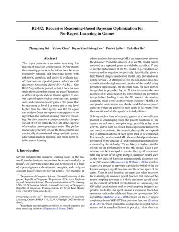
R2-B2: Recursive Reasoning-Based Bayesian Optimization for No-Regret Learning in Lv000 (R2-B2-Lite)1250100IterationsAttack ScoreMean 0(a) common-payoff gamesvs.vs.vs.vs.vs.vs.vs.LvLvLvLvLvLvLv50000 (R2-B2-Lite)11 (R2-B2-Lite)12100Iterations150(d) random search0.250.5Attack ScoreMean RegretTheorem 3 reveals that R1,T grows sublinearly in T .4 So,A using R2-B2 for level-k 2 reasoning achieves asymp0totic no regret regardless of D’s level-0 strategy P2,t. Bycomparing Theorems 1 and 3, we can observe that if A usesGP-MW as its level-0 strategy, then it can achieve fasterasymptotic convergence to no regret by using R2-B2 to reason at level k 2 and one level higher than D. However,when A reasons at a higher level k, its computational costgrows due to an additional optimization of the GP-UCB acquisition function per increase in level of reasoning. So, Ais expected to favor reasoning at a lower level, which agreeswith the observation in the work of Camerer et al. (2004) onthe cognitive hierarchy model that humans usually reason ata level no higher than 2.0.40.300.200.150.100.0550100Iterations1500(b) general-sum games50100Iterations150(e) GP-MWWe also propose a computationally cheaper variant of R2B2 for level-1 reasoning called R2-B2-Lite at the expense ofa weaker convergence guarantee. When using R2-B2-Litefor level-1 reasoning, instead of following (3), A selects itse02,t from level-0 strategylevel-1 action x11,t by sampling x0P2,t of D and best-responding to this sampled action:e02,t ) .x11,t , arg maxx1 X1 α1,t (x1 , x(8)Our final main result (its proof is in Appendix D) bounds theexpected regret of A using R2-B2-Lite for level-1 reasoning:Theorem 4. Let δ (0, 1). Suppose that A uses R2B2-Lite for level-1 reasoning and D uses mixed strat0egy P2,tfor level-0 reasoning. If the trace of the co0variance matrix of x02,t P2,tis not more than ωt fort 1, . . . , T , Pthen with probabilityof at least 1 δ, TE[R1,T ] O( t 1 ωt T βT γT ) where the expectation is with respect to the history of actions selected ande02,t for t 1, . . . , T .payoffs observed by D as well as xFrom Theorem 4, the expected regret bound tightens if D’s0level-0 mixed strategy P2,thas a smaller variance for eachdimension of input action x02,t . As a result, the level-0 ace02,t of D that is sampled by A tends to be closer totion xthe true level-0 action x02,t selected by D. Then, A canselect level-1 action x11,t that best-responds to a more pree02,t of the level-0 action x02,t selected by D,cise estimate xhence improving its expected payoff. Theorem 4 also reveals that A using R2-B2-Lite for level-1 reasoning achievesasymptotic no expected regret if the sequence (ωt )t Z uniformly decreases to 0 (i.e., ωt 1 ωt for t Z andlimT ωT 0). Interestingly, such a sufficient conditionfor achieving asymptotic no expected regret has a natural and elegant interpretation in terms of the explorationexploitation trade-off: This condition is satisfied if D uses a0level-0 mixed strategy P2,twith a decreasing variance foreach dimension of input action x02,t , which corresponds totransitioning from exploration (i.e., a large variance results0.5Attack Score3.2. R2-B2-LiteMean c) constant-sum games5075100Iterations125150(f)Figure 2. (a-c) Mean regret of agent 1 in synthetic games wherethe legend in (a) represents the levels of reasoning of agents 1vs. 2. Attack score of A in adversarial ML for (d-e) MNIST and(f) CIFAR-10 datasets where the legend in (d) represents the levelsof reasoning of A vs. D.0in a diffused P2,tand hence many actions being sampled) to0exploitation (i.e., a small variance results in a peaked P2,tand hence fewer actions being sampled).4. Experiments and DiscussionThis section empirically evaluates the performance of ourR2-B2 algorithm and demonstrates its generality using synthetic games, adversarial ML, and MARL. Some of ourexperimental comparisons can be interpreted as comparisons with existing baselines used as level-0 strategies (Section 3.1.1). Specifically, we can compare the performance ofour level-1 agent with that of a baseline method when theyare against the same level-0 agent. Moreover, in constantsum games, we can perform a more direct comparison byplaying our level-1 agent against an opponent using a baseline method as a level-0 strategy (Section 4.2.2). Additionalexperimental details and results are reported in Appendix Fdue to lack of space. All error bars represent standard error.4.1. Synthetic GamesFirstly, we empirically evaluate the performance of R2-B2using synthetic games with two agents whose payoff functions are sampled from GP over a discrete input domain.Both agents use GP-MW and R2-B2/R2-B2-Lite for level-
R2-B2: Recursive Reasoning-Based Bayesian Optimization for No-Regret Learning in Games0 and level-k 1 reasoning, respectively. We consider 3types of games: common-payoff, general-sum, and constantsum games. Figs. 2a to 2c show results of the mean regret5of agent 1 averaged over 10 random samples of GP and 5initializations of 1 randomly selected action with observedpayoff per sample: In all types of games, when agent 1reasons at one level higher than agent 2, it incurs a smallermean regret than when reasoning at level 0 (blue curve),which demonstrates the performance advantage of recursivereasoning and corroborates our theoretical results (Theorems 2 and 3). The same can be observed for agent 1 usingR2-B2-Lite for level-1 reasoning (orange curve) but it doesnot perform as well as that using R2-B2 (red curve), whichagain agrees with our theoretical result (Theorem 4). Moreover, comparing the red (orange) and blue curves showsthat when against the same level-0 agent, our R2-B2 (R2B2-Lite) level-1 agent outperforms the baseline method ofGP-MW (as a level-0 strategy).Figs. 2a and 2c also reveal the effect of incorrect thinking ofthe level of reasoning of the other agent on its performance:Since agent 2 uses recursive reasoning at level 1 or more,agent 2 thinks that it is reasoning at one level higher thanagent 1. However, it is in fact reasoning at one level lowerin these two figures. In common-payoff games, since agents1 and 2 have identical payoff functions, the mean regret ofagent 2 is the same as that of agent 1 in Fig. 2a. So, fromagent 2’s perspective, it benefits from such an incorrectthinking in common-payoff games. In constant-sum games,since the payoff function of agent 2 is negated from thatof agent 1, the mean regret of agent 2 increases with adecreasing mean regret of agent 1 in Fig. 2c. So, from agent2’s viewpoint, it hurts from such an incorrect thinking inconstant-sum games. Further experimental results on suchincorrect thinking are reported in Appendix F.1.1b.An intriguing observation from Figs. 2a to 2c is that whenagent 1 reasons at level k 2, it incurs a smaller meanregret than when reasoning at level 1. A possible explanation is that when agent 1 reasons at level k 2, its selectedlevel-k action (6) best-responds to the actual level-(k 1)action (7) selected by agent 2. In contrast, when agent 1reasons at level 1, its selected level-1 action (3) maximizesthe expected value of GP-UCB w.r.t. agent 2’s level-0 mixedstrategy rather than the actual level-0 action selected byagent 2. However, as we shall see in the experiments onadversarial ML in Section 4.2.1, when the expectation inlevel-1 reasoning (3) needs to be approximated via sampling but insufficient samples are used, the performance oflevel-k 2 reasoning can be potentially diminished due topropagation of the approximation error from level 1.PThe mean regret T 1 Tt 1 (maxx1 X1 ,x2 X2 f1 (x1 , x2 ) f1 (x1,t , x2,t )) of agent 1 pessimistically estimates (i.e., upperbounds) R1,T /T (1) and is thus not expected to converge to 0.Nevertheless, it serves as an appropriate performance metric here.5Moreover, Fig. 2c shows another interesting observationthat is unique for constant-sum games: Agent 1 achieves asignificantly better performance when reasoning at level 3(i.e., agent 2 reasons at level 2) than at level 2 (i.e., agent2 reasons at level 1). This can be explained by the factthat when agent 2 reasons at level 2, it best-responds tothe level-1 action of agent 1, which is most likely differentfrom the actual action selected by agent 1 since agent 1is in fact reasoning at level 3. In contrast, when agent 2reasons at level 1, instead of best-responding to a single(most likely wrong) action of agent 1, it best-responds to theexpected behavior of agent 1 by attributing a distributionover all actions of agent 1. As a result, agent 2 suffers froma smaller performance deficit when reasoning at level 1 (i.e.,agent 1 reasons at level 2) compared with reasoning at level2 (i.e., agent 1 reasons at level 3) or higher. Therefore, agent1 obtains a more dramatic performance advantage whenreasoning at level 3 (gray curve) due to the constant-sumnature of the game. A deeper implication of this insightis that although level-1 reasoning may not yield a betterperformance than level-k 2 reasoning as analyzed inthe previous p
At level k 0 of reasoning, the agent randomizes its choice of actions. At a higher level k 1 of reasoning, the agent selects its best response to the actions of the other agents who are reasoning at lower levels 0;1;:::;k 1. This paper presents the first recursive reasoning formalism of BO to model the reasoning process in the interactions