WIXLIB

https://www.halvorsen.blogDifferential Equationsin PythonHans-Petter Halvorsen

Free Textbook with lots of Practical amming/python/

Additional Python ramming/python/

Contents Differential EquationsSimulationODE SolversDiscrete SystemsTo benefit from the tutorial, you shouldExamplesalready know about differential equations

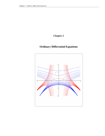
Python Editors Python IDLESpyder (Anaconda distribution)PyCharmVisual Studio CodeVisual StudioJupyter Notebook

Spyder (Anaconda distribution)Run Program buttonVariable Explorer windowCode Editor windowConsole windowhttps://www.anaconda.com

https://www.halvorsen.blogDifferential EquationsHans-Petter Halvorsen

Differential EquationsDifferential Equation on general form:𝑑𝑦 𝑓 𝑡, 𝑦 ,𝑑𝑡Different notation is used:𝑦 𝑡! 𝑦!Example:𝑑𝑦 𝑦 ! 𝑦̇𝑑𝑡ODE – Ordinary Differential EquationsInitial condition𝑑𝑦 3y 2,𝑑𝑡𝑦 𝑡! 0

Differential EquationsExample: %Note that 𝑥̇ &Where 𝑥! 𝑥 0 𝑥(𝑡! ) is the initial condition𝑥̇ 𝑎𝑥"Where 𝑎 #, where 𝑇 is denoted as the time constant of the systemThe solution for the differential equation is found to be (learnedin basic Math courses):𝑥 𝑡 𝑒 !" 𝑥#Where 𝑥! 𝑥 0 𝑥(𝑡! ) is the initial condition

Python Code𝑥 𝑡 𝑒 -& 𝑥.In our system we can set 𝑇 5 andthe initial condition 𝑥! 𝑥(0) 1import math as mtimport numpy as npimport matplotlib.pyplot as plt# ParametersT 5a -1/Tx0 1t 0tstart 0tstop 25increment 1x []x np.zeros(tstop 1)t np.arange(tstart,tstop 1,increment)# Define the Equationfor k in range(tstop):x[k] mt.exp(a*t[k]) * x0# Plot the Resultsplt.plot(t,x)plt.title('Plotting Differential Equation d()plt.axis([0, 25, 0, 1])

Alt. Solution𝑥 𝑡 𝑒 -& 𝑥.In our system we can set 𝑇 5 andthe initial condition 𝑥! 𝑥(0) 1In this alternative solution noFor Loop has been usedimport numpy as npimport matplotlib.pyplot as plt# ParametersT 5a -1/Tx0 1t 0tstart 0tstop 25increment 1N 25#t np.arange(tstart,tstop 1,increment)#Alternative Approacht np.linspace(tstart, tstop, N)x np.exp(a*t) * x0# Plot the Resultsplt.plot(t,x)plt.title('Plotting Differential Equation d()plt.axis([0, 25, 0, 1])plt.show()

Comments to Example Solving differential equations like shown in theseexamples works fine But the problem is that we first have to manually (by“pen and paper”) find the solution to the differentialequation. An alternative is to use solvers for Ordinary DifferentialEquations (ODE) in Python, so-called ODE Solvers The next approach is to find the discrete version andthen implement and simulate the discrete system

ODE Solvers in Python The scipy.integrate library has two powerful powerfulfunctions; ode() and odeint(), for numerically solving firstorder ordinary differential equations (ODEs). The ode() is more flexible, while odeint() (ODE integrator)has a simpler Python interface and works fine for mostproblems. For details, see the SciPy documentation: ed/scipy.integrate.odeint.html enerated/scipy.integrate.ode.html

Python CodeHere we use an ODE solver in SciPy𝑥̇ 𝑎𝑥In our system we can set 𝑇 5 andthe initial condition 𝑥! 𝑥(0) 1import numpy as npfrom scipy.integrate import odeintimport matplotlib.pyplot as plt# Initializationtstart 0tstop 25increment 1x0 1t np.arange(tstart,tstop 1,increment)# Function that returns dx/dtdef mydiff(x, t):T 5a -1/Tdxdt a * xreturn dxdt# Solve ODEx odeint(mydiff, x0, t)print(x)# Plot the Resultsplt.plot(t,x)plt.title('Plotting Differential Equation d()plt.axis([0, 25, 0, 1])plt.show()

Passing Argument𝑥̇ 𝑎𝑥!We set 𝑇 5, 𝑎 " and 𝑥# 𝑥(0) 1In the modified example we have theparameters used in the differential equation(in this case a) as an input argument.By doing this, it is very easy to changevalues for the parameters used in thedifferential equation without changing thecode for the differential equation.The differential equation can even be in aseparate file.import numpy as npfrom scipy.integrate import odeintimport matplotlib.pyplot as plt# InitializationT 5a -1/Ttstart 0tstop 25increment 1x0 1t np.arange(tstart,tstop 1,increment)# Function that returns dx/dtdef mydiff(x, t, a):dxdt a * xreturn dxdt# Solve ODEx odeint(mydiff, x0, t, args (a,))print(x)# Plot the Resultsplt.plot(t,x)plt.title('Plotting Differential Equation d()plt.axis([0, 25, 0, 1])plt.show()

Passing ArgumentsPython CommentsYou can also easily run multiplesimulations like this:Then you can run multiplesimulations for different values of a.a -0.2x odeint(mydiff, x0, t, args (a,))a -0.1x odeint(mydiff, x0, t, args (a,)).To write a tuple containing a single value you have toinclude a comma, even though there is only one valueargs (a,)

Diff. Eq. in Separate .py File“differential equations.py“:def mydiff1(x, t, a):dxdt a * xreturn dxdt“test mydiffq.py“:from differential equations import mydiff1import numpy as npfrom scipy.integrate import odeintimport matplotlib.pyplot as plt# InitializationT 5a -1/Ttstart 0tstop 25increment 1x0 1t np.arange(tstart,tstop 1,increment)# Solve ODEx odeint(mydiff1, x0, t, args (a,))print(x)# Plot the Resultsplt.plot(t,x)plt.title('Plotting Differential Equation d()plt.axis([0, 25, 0, 1])plt.show()

Diff. Eq. in For Loop𝑥̇ 𝑎𝑥“differential equations.py“:"Where 𝑎 , where def mydiff1(x, t, a):#dxdt a * x𝑇 is denoted as thereturn dxdttime constant of thesystemfrom differential equations import mydiff1import numpy as npfrom scipy.integrate import odeintimport matplotlib.pyplot as plt# InitializationTsimulations [2, 5, 10, 20]tstart 0tstop 25increment 1x0 1t np.arange(tstart,tstop 1,increment)for T in Tsimulations:a -1/T# Solve ODEx odeint(mydiff1, x0, t, args (a,))print(x)# Plot the Resultsplt.plot(t,x)“test mydiffq.py“:plt.title('Plotting dxdt d()plt.axis([0, 25, 0, 1])plt.legend(["T 2", "T 5", "T 10", "T 20"])plt.show()

r Halvorsen

DiscretizationThe differential equation of the system is:𝑥̇ 𝑎𝑥Next:𝑥 %" 𝑥 𝑇& 𝑎𝑥 We need to find the discrete version:Next:We use the Euler forward method:𝑥"# 𝑥"𝑥̇ 𝑇%𝑥56" 𝑥5 𝑇7 𝑎𝑥5This gives:𝑥 %" 𝑥 𝑎𝑥 𝑇&This gives the following discrete version:𝑥56" (1 𝑎𝑇7 ) 𝑥5

Python CodeDifferential Equation: 𝒙̇ 𝒂𝒙Simulation of Discrete System:𝒙𝒌%𝟏 (𝟏 𝒂𝑻𝒔 )𝒙𝒌import numpy as npimport matplotlib.pyplot as plt# Model ParametersT 5a -1/T# Simulation ParametersTs 0.01Tstop 25N int(Tstop/Ts) # Simulation lengthx np.zeros(N 2) # Initialization the x vectorx[0] 1 # Initial Condition# Simulationfor k in range(N 1):x[k 1] (1 a*Ts) * x[k]# Plot the Simulation Resultst np.arange(0,Tstop 2*Ts,Ts) # Create Time Seriesplt.plot(t,x)plt.title('Plotting Differential Equation d()plt.axis([0, 25, 0, 1])plt.show()

Discretization Discretization are covered more in detail inanother Tutorial/Video You find also more aboutDiscretization in my Textbook“Python for Science nts/programming/python/

https://www.halvorsen.blogMore ExamplesHans-Petter Halvorsen

Bacteria SimulationIn this example we will simulate a simple model of a bacteria population in a jar.The model is as follows:Birth rate: 𝑏𝑥Death rate: 𝑝𝑥 *Then the total rate of change of bacteria population is:𝑥̇ 𝑏𝑥 𝑝𝑥 ?Where x is the number of bacteria in the jarNote that 𝑥̇ ,We will simulate the number of bacteriain the jar after 1 hour, assuming thatinitially there are 100 bacteria present. -In the simulations we can set b 1/hour and p 0.5 bacteria-hour

Python CodeDifferential Equation: 𝑥̇ 𝑏𝑥 𝑝𝑥 &import numpy as npfrom scipy.integrate import odeintimport matplotlib.pyplot as plt# Initializationtstart 0tstop 1increment 0.01x0 100t np.arange(tstart,tstop increment,increment)# Function that returns dx/dtdef bacteriadiff(x, t):b 1p 0.5dxdt b * x - p * x**2return dxdt# Solve ODEx odeint(bacteriadiff, x0, t)#print(x)# Plot the Resultsplt.plot(t,x)plt.title('Bacteria rid()plt.axis([0, 1, 0, 100])plt.show()

Simulation with 2 variablesGiven the following system:𝑑𝑥" 𝑥?𝑑𝑡𝑑𝑥? 𝑥"𝑑𝑡Let's simulate the system in Python. The equations will besolved in the time span [ 1 1] with initial values [1, 1].

Python CodeSystem:𝑑𝑥" 𝑥*𝑑𝑡𝑑𝑥* 𝑥"𝑑𝑡import numpy as npfrom scipy.integrate import odeintimport matplotlib.pyplot as plt# Initializationtstart -1tstop 1increment 0.1x0 [1,1]t np.arange(tstart,tstop 1,increment)# Function that returns dx/dtdef mydiff(x, t):dx1dt -x[1]dx2dt x[0]dxdt [dx1dt,dx2dt]return dxdt# Solve ODEx odeint(mydiff, x0, t)print(x)x1 x[:,0]x2 x[:,1]# Plot the lation with 2 id()plt.axis([-1, 1, -1.5, 1.5])plt.legend(["x1", "x2"])plt.show()

https://www.halvorsen.blogSimulation of1.order SystemHans-Petter Halvorsen

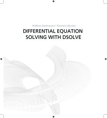
1.order Dynamic SystemAssume the following general Differential Equation:Input Signal𝑦̇ 𝑎𝑦 𝑏𝑢𝑢(𝑡)or𝑦̇ 1( 𝑦 𝐾𝑢)𝑇Where 𝑎 "#and 𝑏 DynamicSystemOutput Signal𝑦(𝑡).#Where 𝐾 is the Gain and 𝑇 is the Time constantThis differential equation represents a 1. order dynamic systemAssume 𝑢(𝑡) is a step (𝑈), then we can find that the solution to the differential equation is:𝑦 𝑡 𝐾𝑈(1 𝑒/#)

Step Response𝐾𝑈100%63%𝑦̇ 1( 𝑦 𝐾𝑢)𝑇𝑦 𝑡 𝐾𝑈(1 𝑒/#)𝑡𝑇

1.order Dynamic System1( 𝑦 𝐾𝑢)𝑇Let's find the mathematical expression for the step response𝐾We use Laplace:𝑦𝑠 𝑢(𝑠)Note 𝑦̇ 𝑠𝑦(𝑠)𝑇𝑠 10We apply a step in the input signal 𝑢(𝑠): 𝑢 𝑠 1&𝑠𝑦(𝑠) ( 𝑦(𝑠) 𝐾𝑢(𝑠))𝐾𝑈𝑇𝑦 𝑠 HNext, we use Inverse Laplace𝑇𝑠 1 𝑠1𝐾𝑠𝑦 𝑠 𝑦(𝑠) 𝑢(𝑠)We use the following Laplace Transformation pair𝑇𝑇𝑘in order to find 𝑦(𝑡):/# 𝑘(1 𝑒 )𝑇𝑠𝑦 𝑠 𝑦(𝑠) 𝐾𝑢(𝑠)𝑇𝑠 1 𝑠This gives the following step response:(𝑇𝑠 1)𝑦 𝑠 𝐾𝑢(𝑠)/#𝑦 𝑡 𝐾𝑈(1 𝑒 )Given the differential equation: 𝑦̇

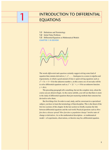
Python CodeWe start by plotting the following:𝑦 𝑡 &J#𝐾𝑈(1 𝑒 )In the Python code we can set:𝑈 1𝐾 3𝑇 4import numpy as npimport matplotlib.pyplot as pltK 3T 4start 0stop 30increment 0.1t np.arange(start,stop,increment)y K * (1-np.exp(-t/T))plt.plot(t, y)plt.title('1.order Dynamic System')plt.xlabel('t [s]')plt.ylabel('y(t)'plt.grid()

Python Code1𝑦̇ ( 𝑦 𝐾𝑢)𝑇In the Python code we can set:𝐾 3𝑇 4import numpy as npfrom scipy.integrate import odeintimport matplotlib.pyplot as plt# InitializationK 3T 4u 1tstart 0tstop 25increment 1y0 0t np.arange(tstart,tstop 1,increment)# Function that returns dx/dtdef system1order(y, t, K, T, u):dydt (1/T) * (-y K*u)return dydt# Solve ODEx odeint(system1order, y0, t, args (K, T, u))print(x)# Plot the Resultsplt.plot(t,x)plt.title('1.order System dydt (1/T)*(-y lt.show()

Additional Python ramming/python/

Hans-Petter HalvorsenUniversity of South-Eastern Norwaywww.usn.noE-mail: hans.p.halvorsen@usn.noWeb: https://www.halvorsen.blog

Python Code import numpyas np import matplotlib.pyplotas plt K 3 T 4 start 0 stop 30 increment 0.1 t np.arange(start,stop,increment) y K * (1-np.exp(-t/T)) plt.plot(t, y) plt.title('1.order Dynamic System') plt.xlabel('t [s]') plt.ylabel('y(t)' plt.grid() "# 67(1 *J & #) We start by plotting the following: In the Python code we .