WIXLIB

1.1. ROW OPERATIONS21.1.1 Definition. Applied to the augmented matrix a11 a12 . . . a1n a21 a22 . . . a2n A0 . .am1 am2 . . . b1b2 . . (1.1.2)amn bmthese operations have the following effect:1. Multiplying a row of A0 by a non-zero number;2. Interchanging the rows of A0 ;3. Adding to a row of A0 a multiple of another row.They are called row operations.Using only these three matrix operations, we will put the coefficient matrix Ainto row echelon form. Recall that Ai denotes the i-th row of A.1.1.3 Definition. The matrix A is in row echelon form if1. All the rows of A that consist entirely of zeroes are below any row of A thathas a non-zero entry;2. If row Ai has its first non-zero entry in position j, then row Ai 1 has its firstnon-zero entry in position j.1.1.4 Remark. This definition implies that the first non-zero entry of Ai in a position j i. Thus if A is in row echelon form, aij 0 for all j i. If A is square,this means that A is upper triangular.1.1.5 Example. The matrices 1 2 30 2 3 1 2 3 0 4 0 , 0 0 2 , and 0 2 2 0 0 10 0 000 0are in row echelon form, while 1 2 30 2 30 0 3 0 4 0 , 0 0 0 , and 0 0 2 0 2 10 0 10 0 1are not.The central theorem is1.1.6 Theorem. Any matrix can be put in row echelon form by using only rowoperations.

1.2. ELEMENTARY MATRICES3Proof. We prove this by induction on the number of rows of the matrix A. If A hasone row, there is nothing to prove.So assume the result for matrices with m 1 rows, and let A be a matrix withm rows. If the matrix is the 0 matrix, we are done. Otherwise consider the firstcolumn Ak of A that has a non-zero element. Then for some i, aik 6 0, and for allj k, the column Aj is the zero vector.Since Ak has non-zero entry aik , interchange rows 1 and i of A. So the newmatrix A has a1k 6 0. Then if another row Ai of A has k-th entry aik 6 0, replacethat row byaikAi A1a1kwhich has j-th entry equal to 0. Repeat this on all rows that have a non-zeroelement in column k. The new matrix, which we still call A, has only zeroes in itsfirst k columns except for a1k .Now consider the submatrix B of the new matrix A obtained by removing thefirst row of A and the first k columns of A. Then we may apply the inductionhypothesis to B and put B in row echelon form by row operations. The key observation is that these same row operations may be applied to A, and do not affectthe zeroes in the first k columns of A, since the only non-zero there is in row 1 andthat row has been removed from B.We could of course make this proof constructive by repeating to B the rowoperations we did on A, and continuing in this way.1.1.7 Exercise. Reduce the matrices in Example 1.1.5 that are not already in rowechelon form to row echelon form.At this point we defer the study of the inhomogeneous equation Ax b. Wewill pick it up again in §7.2 when we have more tools.1.2Elementary MatricesFollowing Lang [3], Chapter II §5, we introduce the three types of elementarymatrices, and show they are invertible.In order to do that we let Irs be the square matrix with a irs 1, and zeroeseverywhere else. So for example in the 3 3 case 0 0 0I23 0 0 1 0 0 0

1.2. ELEMENTARY MATRICES41.2.1 Definition. Elementary matrices E are square matrices, say m m. Wedescribe what E does to a matrix m n A when we left-multiply E by A, and wewrite the formula for E. There are three types.1. E multiplies a row of a matrix by a number c 6 0; The elementary matrixEr (c) : I (c 1)Irrmultiplies the r-th row of A by c.2. E interchange two rows of any matrix A; We denote by Trs , r 6 s thepermutation matrix that interchanges row i of A with row j. This is a specialcase of a permutation matrix: see §3.3 for the 3 3 case. The permutationis a transposition.3. E adds a constant times a row to another row; The matrixErs (c) : I cIrs , r 6 s,adds c times the s-th row of A to the r-th row of A.1.2.2 Example. Here are some 3 3 examples, acting on the 3 n matrix a11 . . . a1nA a21 . . . a2n .a31 . . . a3nFirst, since c 0 0E1 (c) 0 1 1 ,0 0 1matrix multiplication gives ca11 . . . E1 (c)A a21 . . .a31 . . .Next since ca1na2n .a3n T23 1 0 0 0 0 1 0 1 0we get a11 . . .T23 A a31 . . .a21 . . . a1na3n .a2n

1.3. ELIMINATION VIA MATRICES5Finally, since 1 0 cE13 (c) 0 1 0 0 0 1we get a11 ca31 . . .a21.E13 (c)A a31. a1n ca33 .a2na3n1.2.3 Theorem. All elementary matrices are invertible.Proof. For each type of elementary matrix E we write down an inverse, namely amatrix F such that EF I F E.For Ei (c) the inverse is Ei (1/c). Tij is its own inverse. Finally the inverse ofEij (c) is Eij ( c).1.3Elimination via MatricesThe following result follows immediately from Theorem 1.1.6 once one understands left-multiplication by elementary matrices.1.3.1 Theorem. Given any m n matrix A, one can left multiply it by elementarymatrices of size m to bring into row echelon form.We are interested in the following1.3.2 Corollary. Assume A is a square matrix of size m. Then we can left-multiplyA by elementary matrices Ei , 1 i k until we reach either the identity matrix,or a matrix whose bottom row is 0. In other words we can writeA0 Ek . . . E1 A.(1.3.3)where either A0 I or the bottom row of A0 is the zero vector.Proof. Using Theorem 1.3.1, we can bring A into row echelon form. Call the newmatrix AB. As we noted in Remark 1.1.4 this means that B is upper triangular.If any diagonal entry bii of B is 0, then the bottom row of B is zero, and we havereached one of the conclusions of the theorem.So we may assume that all the diagonal entries of B are non-zero. We now dowhat is called backsubstitution to transform B into the identity matrix.First we left multiply by the elementary matricesEm (1/bmm ), Em 1 (1/bm 1,m 1 ), . . . , E1 (1/b11 )

1.3. ELIMINATION VIA MATRICES6. This new matrix, that we still call B, now has 1s along the diagonal.Next we left multiply by elementary matrices of type (3) in the orderEm,m 1 (c),Em,m 2 (c), . . . , Em,1 (c),Em 1,m 2 (c),Em 1,m 3 (c), . . . , Em 1,1 (c),.,.E2,1 (c).where in each case the constant c is chosen so that a new zero in created in the matrix. This order is chosen so that no zeroes created by a multiplication is destroyedby a subsequent one. At the end of the process we get the identity matrix I so weare done.1.3.4 Exercise. Reduce the matrices in Example 1.1.5 either to a matrix with bottom row zero or to the identiy matrix using left multiplcation by elementary matrices.For example, the first matrix 1 2 3 0 4 0 0 0 1backsubstitutes to 1 2 31 2 01 0 0 0 1 0 , then 0 1 0 , then 0 1 0 .0 0 10 0 10 0 1We will use these results on elementary matrices in §2.2 and then throughoutChapter 8.

Chapter 2Matrix InversesThis chapter fill in some gaps in the exposition in Lang, especially the break between his more elementary text [3] and the textbook [4] we use. There are someadditional results: Proposition 2.2.5 and Theorem 2.2.8. They will be importantlater.2.1BackgroundOn page 35 of our text [4], Lang gives the definition of an invertible matrix.2.1.1 Definition. A n n matrix A is invertible if there exists another n n matrixB such thatAB BA I.(2.1.2)We say that B is both a left inverse and a right inverse for A. It is reasonableto require both since matrix multiplication is not commutative. Then Lang proves:2.1.3 Theorem. If A has an inverse, then its inverse B is unique.Proof. Indeed assume there is another matrix C satisfying (2.1.2) when C replacesB. ThenC CI C(AB) (CA)B IB B(2.1.4)so we are done.Note that the proof only uses that C is a left inverse and B a right inverse.We say, simply, that B is the inverse of A and A the inverse of B.In [4], on p. 86, Chapter IV, §2, in the proof of Theorem 2.2, Lang only establishes that a certain matrix A has a left inverse, when in fact he needs to show ithas an inverse. We recall this theorem and its proof in 4.1.4. We must prove that

2.2. MORE ELIMINATION VIA MATRICES8having a left inverse is enough to get an inverse. Indeed, we will establish this inTheorem 2.2.8.2.2More Elimination via MatricesIn 1.2.1 we introduced the three types of elementary matrices and showed they areinvertible in Theorem 1.2.3.2.2.1 Proposition. Any product of elementary matrices is invertible.Proof. This follows easily from a more general result. Let A and B are two invertible n n matrices, with inverses A 1 and B 1 . Then B 1 A 1 in the inverse ofABIndeed just computeB 1 A 1 AB B 1 IB B 1 B IandABB 1 A 1 A 1 IA A 1 A I.Before stating the next result, we make a definition:2.2.2 Definition. Two m n matrices A and B are row equivalent if there is aproduct of elementary matrices E such that B EA.By Proposition 2.2.1 E is invertible, so if B EA, then A E 1 B.2.2.3 Proposition. If A is a square matrix, , and if B is row equivalent to A, thenA has an inverse if and only if B has an inverse.Proof. Write B EA. If A is invertible, then A 1 E 1 is the inverse of B. Weget the other implication by symmetry.2.2.4 Remark. This establishes an equivalence relation on m n matrices, asdiscussed in §4.3.We continue to assume that A is a square matrix. Corollary 1.3.2 tells us thatA is either row equivalent to the identity matrix I, in which case it is obviouslyinvertible by Proposition 2.2.3, or row equivalent to a matrix with bottom row thezero vector.

2.2. MORE ELIMINATION VIA MATRICES92.2.5 Proposition. Let A be a square matrix with one row equal to the zero vector.Then A is not invertible.Proof. By [4] , Theorem 2.1 p. 30, the homogeneous systemAX O(2.2.6)has a non-trivial solution X, since one equation is missing, so that the number ofvariables is greater than the number of equations. But if A were invertible, wecould multiply (2.2.6) on the left by A 1 to get A 1 AX A 1 O. This yieldsX O, implying there cannot be a non-trivial solution, a contradiction to theassumption that A is invertible.Proposition 5.1.4 generalizes this result to matrices that are not square.So we get the following useful theorem. The proof is immediate.2.2.7 Theorem. A square matrix A is invertible if and only if it is row equivalentto the identity I. If it is not invertible, it is row equivalent to a matrix whose lastrow is the zero vector. Furthermore any upper triangular matrix square A withnon-zero diagonal elements is invertible.Finally, we get to the key result of this section.2.2.8 Theorem. Let A be a square matrix which has a left inverse B, so thatBA I. Then A is invertible and B is its inverse.Similarly, if A has a right inverse B, so that AB I, the same conclusionholds.Proof. Suppose first that AB I, so B is a right inverse. Perform row reductionon A. By Theorem 2.2.7, there are elementary matrices E1 , E2 , . . . , Ek so thatthe row reduced matrix A0 Ek . . . E1 A is the identity matrix or has bottom rowzero. Then multiply by B on the right and use associativity:A0 B (Ek . . . E1 A)B (Ek . . . E1 )(AB) Ek . . . E1 .This is invertible, because elementary matrices are invertible, so all rows of A0 Bare non-zero by Proposition 2.2.5. Now if A0 had a zero row, matrix multiplicationtells us that A0 B would have a zero row, which is impossible. So A0 I. FinallyProposition 2.2.3 tells us that A is invertible, since it is row equivalent to I. Inparticular its left inverse Ek . . . E1 and its right inverse B are equal.To do the direction BA I, just interchange the role of A and B.

2.3. INVERTIBLE MATRICES102.2.9 Remark. The first five chapters of Artin’s book [1] form a nice introductionto linear algebra at a slightly higher level than Lang’s, with some group theorythrown in too. The main difference is that Artin allows his base field to be anyfield, including a finite field, while Lang only allows R and C. The references toArtin’s book are from the first edition.2.3Invertible MatricesThe group (for matrix multiplication) of invertible square matrices has a name: thegeneral linear group, written Gl(n). Its dimension is n2 . Most square matrices areinvertible, in a sense one can make precise, for example by a dimension count. Asingle number, the determinant of A, tells us if A is invertible or not, as we willfind out in [4], Chapter VI.It is worth memorizing what happens in the 2 2 case. The matrixA a b c dis invertible if and only if ad bc 6 0, in which case the inverse of A isA 11 d b ad bc c aas you should check by direct computation. See Exercise 4 of [I, §2].

Chapter 3Groups and PermutationMatricesIn class we studied the motions of the equilateral triangle whose center of gravity isat the origin of the plane, so that the three vertices are equidistant from the origin.We set this up so that one side of the triangle is parallel to the x- axis. There are6 3! motions of the triangle permuting the vertices, and they can be realized bylinear transformations, namely multiplication by 2 2 matrices.These notes describe these six matrices and show that they can be multipliedtogether without ever leaving them, because they form a group: they are closedunder matrix multiplication. The multiplication is not commutative, however. Thisis the simplest example of a noncommutative group, and is worth remembering.Finally, this leads us naturally to the n n permutation matrices. We will see in§3.3 that they form a group. When n 3 it is isomorphic to the group of motionsof the equilateral triangle. From the point of view of linear algebra, permutationand permutation matrices are the most important concepts of these chapter. Wewill need them when we study determinants.There are some exercises in this chapter. Lots of good practice in matrix multiplication.3.1The Motions of the Equilateral TriangleThe goal of this section is to write down six 2 2 matrices such that multiplicationby those matrices induce the motions of the equilateral triangle.First the formal definition of a permutation:3.1.1 Definition. A permutation σ of a finite set S is a bijective map from S toitself. See [4], p. 48.

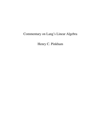
3.1. THE MOTIONS OF THE EQUILATERAL TRIANGLE12We are interested in the permutations of the vertices of the triangle. Becausewe will be realizing these permutations by linear transformations and because thecenter of the triangle is fixed by all linear transformations, it turns out that eachlinear transformation fixes the entire triangle. Here is the graph.θ 1200300orMirrMirrorY AxisPX AxisQRLeft-Right MirrorTo start, we have the identity motion given by the identity matrix 1 0I .0 1Next the rotations. Since the angle of rotation is 120 degrees, orthe first matrix of rotation is cos 2π sin 2π 1/2 3/233 R1 .sin 2πcos 2π3/2 1/2332π3radians,Lang [4] discusses this on page 85. The second one, R2 , corresponds rotation by240 degrees. You should check directly what R2 is, just like we did for R1 . Youwill get:

3.2. GROUPS13 R2 3/2 1/2 . 3/2 1/2More importantly note that R2 is obtained by repeating R1 , in matrix multiplication:R2 R12 .Also recall Lang’s Exercise 23 of Chapter II, §3.Next let’s find the left-right mirror reflection of the triangle. What is its matrix?In the y coordinate nothing should change, and in the x coordinate, the sign shouldchange. The matrix that does this is 1 0M1 0 1This is an elementary matrix, by the way.One property that all mirror reflection matrices share is that their square is theidentity. True here.Finally, the last two mirror reflections. Here they are. Once you understandwhy conceptually the product is correct, to do the product just change the sign ofthe terms in the first column of R1 and R2 : 1/2 1/23/23/2 and M3 R2 M1 . 3/2 1/23/2 1/2 M2 R1 M1 In the same way, to compute the product M1 R1 just change the sign of theterms in the first row of R1 .3.1.2 Exercise. Check that the squares of M2 and M3 are the identity. Describeeach geometrically: what is the invariant line of each one. In other words, if youinput a vector X R2 , what is M2 X, etc.3.2Groups3.2.1 Exercise. We now have six 2 2 matrices, all invertible. Why? The nextexercise will give an answer.3.2.2 Exercise. Construct a multiplication table for them. List the 6 elements inthe order I, R1 , R2 , M1 , M2 , M3 , both horizontally and vertically, then have theelements in the table you construct represent the product, in the following order: ifA is the row element, and B is the column element, then put AB in the table. See

3.2. Table 3.1: Multiplication Table.Artin [1], chapter II, §1, page 40 for an example, and the last page of these notesfor an unfinished example. The solution is given in Table 3.1.Show that this multiplication is not commutative, and notice that each row andcolumn contains all six elements of the group.Table 3.1 is the solution to the exercise. The first row and the first column ofthe table just give the elements to be multiplied, and the entry in the table give theproduct. Notice that the 6 6 table divides into 4 3 3 subtables, each of whichcontains either M elements or R and I elements, but not both.What is a group? The formal definition is given in Lang in Appendix II.3.2.3 Definition. A group is a set G with a map G G G, written as multiplication, which to a pair (u, v) of elements in G associates uv in G, where this map,called the group law, satisfies three axioms:GP 1. The group law is associative: Given elements u, v and w in G,(uv)w u(vw).GR 2. Existence of a neutral element 1 G for the group law: for every elementu G,1u u1 u.GR 3. Existence of an inverse for every element: For every u G there is a v Gsuch thatuv vu 1.The element v is written u 1 .If you look at the first three axioms of a vector space, given in Lang p.3, youwill see that they are identical. Only two changes: the group law is written likemultiplication, while the law in vector spaces is addition. The neutral element

3.2. GROUPS15for vector spaces is O, while here we write it as 1. These are just changes innotation, not in substance. Note that we lack axiom VP 4, which in our notationwould be written:GR 4. The group law is commutative: For all u and v in Guv vu.So the group law is not required to be commutative, unlike addition in vectorspaces. A group satisfying GR 4 is called a commutative group. So vector spacesare commutative groups for their law of addition.One important property of groups is that cancelation is possible:3.2.4 Proposition. Given elements u, v and w in G,1. If uw vw, then u v.2. If wu wv, then u v again.Proof. For (1) multiply the equation on the right by the inverse of w to get(uw)w 1 (vw)w 1by existence of inverse,u(ww 1 ) v(ww 1 )by associativity,u1 v1u vby properties of inverses,by property of neutral elem

These notes were written to complement and supplement Lang's Linear Algebra [4] as a textbook in a Honors Linear Algebra class at Columbia University. . The book is intended for students having had an elementary course in linear algebra. However, by spending a week on Gaussian elimination after covering the second chapter of [4], it was .