Transcription
Recurrent Networks and N ARMA ModelingJerome ConnorLes E. AtlasFT-lOInteractive Systems Design LaboratoryDept. of Electrical EngineeringUniversity of WashingtonSeattle, Washington 98195Douglas R. MartinB-317Dept. of StatisticsUniversity of WashingtonSeattle, Washington 98195AbstractThere exist large classes of time series, such as those with nonlinear movingaverage components, that are not well modeled by feedforward networksor linear models, but can be modeled by recurrent networks. We show thatrecurrent neural networks are a type of nonlinear autoregressive-movingaverage (N ARMA) model. Practical ability will be shown in the results ofa competition sponsored by the Puget Sound Power and Light Company,where the recurrent networks gave the best performance on electric loadforecasting.1IntroductionThis paper will concentrate on identifying types of time series for which a recurrentnetwork provides a significantly better model, and corresponding prediction, thana feedforward network. Our main interest is in discrete time series that are parsimoniously modeled by a simple recurrent network, but for which, a feedforwardneural network is highly non-parsimonious by virtue of requiring an infinite amountof past observations as input to achieve the same accuracy in prediction.Our approach is to consider predictive neural networks as stochastic models. Section2 will be devoted to a brief summary of time series theory that will be used toillustrate the the differences between feedforward and recurrent networks. Section 3will investigate some of the problems associated with nonlinear moving average andstate space models of time series. In particular, neural networks will be analyzed as301
302Connor, Atlas, and Martinnonlinear extensions oftraditionallinear models. From the preceding sections, it willbecome apparent that the recurrent network will have advantages over feedforwardneural networks in much the same way that ARMA models have over autoregressivemodels for some types of time series.Finally in section 4, the results of a competition in electric load forecasting sponsored by the Puget Sound Power and Light Company will discussed. In this competition, a recurrent network model gave superior results to feed forward networksand various types of linear models. The advantages of a state space model formultivariate time series will be shown on the Puget Power time series.2Traditional Approaches to Time Series AnalysisThe statistical approach to forecasting involves the construction of stochastic models to predict the value of an observation Xt using previous observations. This isoften accomplished using linear stochastic difference equation models, with randominputs.A very general class of linear models used for forecasting purposes is the class ofARMA(p,q) modelspqXt L PXt-1 L (Jet-i1 1 eti lwhere et denotes random noise, independent of past X" The conditional mean(minimum mean square error) predictor Xt of Xt can be expressed in the recurrentformpqXt L pXt-, L(Jet-i·1 1i lwhere ek is approximated byfk Xk - Xk,Ie t - 1, . , t - qThe key properties of interest for an ARMA(p,q) model are stationarity and invertibility. If the process Xt is stationary, its statistical properties are independent oftime. Any stationary ARMA(p,q) process can be written as a moving average00Xt L hket-k et·k lAn invertible process can be equivalently expressed in terms of previous observationsor residuals. For a process to be invertible, all the poles of the z-transform mustlie inside the unit circle of the z plane. An invertible ARMA(p,q) process can bewritten as an infinite autoregression00Xt L PkXt-k et·k lAs an example of how the inverse process occurs, let et be solved for in terms of Xtand then substitute previous et's into the original process. This can be illustrated
Recurrent Networks and NARMA Modelingwith an MA(I) processXtet-i et (}et-1Xt-i - (}et-i-1 (}(Xt-1 - (}et-2)Xt et (-I)i-1(}iXt iXt etiLooking at this example, it can be seen that an MA(I) processes with I(}I 1 willdepend significantly on observations in the distant past. However, if I(}I 1, thenthe effect of the distant past is negligible.In the nonlinear case, it will be shown that it is not always possible to go backand forth between descriptions in terms of observables (e.g. Xi) and descriptionsin terms of unobservables (e.g. ei) even when St O. For a review of time seriesprediction in greater depth see the works of Box [1] or Harvey [2].3Nonlinear ARMA ModelsMany types of nonlinear models have been proposed in the literature. Here we focuson feed forward and recurrent neural networks and how they relate to nonlinearARMA models.3.1Nonlinear Autoregressive ModelsThe simplest generalization to the nonlinear case would be the nonlinear autoregressive (NAR) modelXt h(xt-1! Xt-2, . , Xt-p) et,where hO is an unknown smooth function with the assumption the best (i.e., minimum mean square error) prediction of Xt given Xt-1I . , Xt-p is its conditional meanZt E(xtl x t-1I . , Xt p)h(xt-1I . , Xt-p).Feedforward networks were first proposed as an NAR model for time series prediction by Lapedes and Farber [3]. A feedforward network is a nonlinear approximationto h given byIZt h(Xt-1I . , Xt-p)p Wd( WijXt-j).i l; 1The weight matrix W is lower diagonal and will allow no feedback. Thus the feedforward network is a nonlinear mapping from previous observation onto predictionsof future observations. The function /(x) is a smooth bounded monotonic function,typically a sigmoid.The parameters Wi and Wij are estimates from a training sample x , . , x')." therebyobtaining an estimate of h of h. Estimates are obtained by minimizing the sumof the square residuals E l (Xt - Zt)2 by gradient descent procedure known as"backpropagation" [4].303
304Connor, Atlas, and Martin3.2NARMA or NMAA simple nonlinear generalization of ARMA models isIt is natural to predictZt h(Xt-b Xt-2, . , Xt-p, et-b . , et-q).If the model h(Xt-b Xt-2, . , Xt-p, et-l, . , et-q) is chosen, then a recurrent networkcan approximate it asZt1pqi 1j 1; 1 h(Xt-1' . , Xt-p) L Wd(L WijXt-j L wij(Xt-j -Zt-j».This model is a special case of the fully interconnected recurrent networkZt 1ni 1j 1L Wd(L wijXt-j)where wij are coefficients of a full matrix.Nonlinear autoregressive models and nonlinear moving average models are not always equivalent for nondeterministic processes as in the linear case. If the probability of the next observation depends on the previous state of the process, arepresentation built on et may not be complete unless some information on the previous state is added[8]. The problem is that if et, . , et-m are known, there is stillnot enough information to determine which state the series is in at t - m. Giventhe lack of knowledge of the initial state, it is impossible to predict future statesand without the state information, the best predictions cannot be made.If the moving average representation cannot be made with et alone, it still may bepossible to express a model in terms of past et and state information.It has been shown that for a large class of nondeterministic Markov processes, amodel of this form can be constructed[8]. This link is important, because a recurrentnetwork is this type of model. For further details on using recurrent networks toNARMA modeling see Connor et al[9].4Competition on Load Forecasting DataA fully interconnected recurrent network trained with the Williams and Zipser algorithm [10] was part of a competition to predict the loads of the Puget Sound Powerand Light Company from November 11, 1990 to March 31, 1991. The object wasto predict the demand for the electric power, known as the load, profile of each dayon the previous working day. Because the forecast is made on Friday morning, theMonday prediction is the most difficult. Actual loads and temperatures of the pastare available as well as forecasted temperatures for the day of the prediction.
Recurrent Networks and NARMA ModelingNeural networks are not parsimonious and many parameters need to be determined.Seasonality limits the amount of useful data for the load forecasting problem. Forexample, the load profile in August is not useful for predicting the load profile inJanuary. This limited amount of data severely constrains the number of parametersa model can accurately determine. We avoided seasonality, while increasing the sizeof the training set by including data form the last four winters. In total 26976vectors were available when data from August 1 to March 31 for 1986 to 1990 wereincluded. The larger training set enables neural network models be trained withless danger of overfitting the data. If the network can accurately model load growthover the years, then the network will have the added advantage of being exposedto a larger temperature spectrum on which to base future predictions. The largertemperature spectrum is hypothetically useful for predicting phenomenon such ascold snaps which can result in larger loads than normal. It should be noted thatneural networks have been applied to this model in the past[6].Initially five recurrent models were constructed, one for each day of the week, withWednesday, Thursday and Friday in a single network. Each network has temperature and load values from a week previous at that hour, the forecasted temperatureof the hour to be predicted, the hour year and the week of the forecast. The week ofthe forecast was included to allow the network to model the seasonality of the data.Some models have added load and temperature from earlier in the week, dependingon the availability of the data. The networks themselves consisted of three to fourneurons in the hidden layer. This predictor is of the formIt(k) et(k - 7) I(lt(k - 7), et(k - 7), it(k), T8(k - 1), t, d, y),where 10 is a nonlinear function, It(k) is the load at time t and day k,is thenoise, T is the temperature, T is the forecasted temperature, d is the day of theweek, and y is the year of the data.etAfter comparing its performance to the winner of the competition, the linear modelin Fig. 1, the poor performance could be attributed to the choice of model, ratherthan a problem with recurrent networks. It should be mentioned that the linearmodel took as one of its inputs, the square of the last available load. This is aparsimonious way of modeling nonlinearities. A second recurrent predictor wasthen built with the same input and output configuration as the linear model, savethe square of the previous load term which the nets nonlinearities can handle. Thisnet, denoted as the Recurrent Network, had a different recurrent model for eachhour of the day. Each hour of the day had a different model, this yielded the bestpredictions. This predictor is of the formIt(k) et(k) It.(lt(k - 1), et(k - 1), it(k), Ts(k - 1), d, y). All of the models in the figure use the last available load, forecasted temperatureat the hour to be predicted, maximum forecasted temperature of the day to bepredicted, the previous midnight temperatures, and the hour and year of the prediction. A second recurrent network was also trained with the last available loadat that hour, this enabled et-l to be modeled. The availability of et-l turned outto be the difference between making superior and average predictions. It should benoted that the use of et-l did not improve the results of linear models.The three most important error measures are the weekly morning, afternoon, andtotal loads and are listed in the table below. The A.M. peak is the mean average305
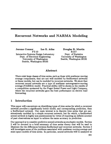
306Connor, Atlas, and MartinRecurrent.0275.0355.0218.0311Table 1: Mean Square Errorpercent error (MAPE) of the summed predictions of 7 A.M. to 9 A.M., the P.M.peak is the MAPE of the summed predictions of 5 P.M. to 7 P.M, and the totalis the MAPE of the summed predictions over the entire day. Results, of the totalpower for the day prediction, of the recurrent network and other predictors areshown in Fig. 1. The performance on the A.M. and P.M. peaks were similar[9].The failure of the daily recurrent network to accurately predict is a product of tryingto model to complex a problem. When the complexity of the problem was reducedto that of predicting a single hour of the day, results improved significantly[7].The superior performance of the recurrent network over the feedforward networkis time series dependent. A feedforward and a recurrent network with the sameinput representation was trained to predict the 5 P.M. load on the previous workday. The feedforward network succeeded in modeling the training set with a meansquare error of .0153 compared to the recurrent networks .0179. However, whenthe tested on several winter outside the training set the results, listed in the tablebelow, varied. For the 1990-91 winter, the recurrent network did better with amean square error of .0311 compared to the feedforward networks .0331. For theother winter of the years before the training set, the results were quite different,the feedforward network won in all cases. The differences in prediction performancecan be explained by the inability of the feedforward network to model load growthin the future. The loads experience in the 1990-91 winter were outside the range ofthe entire training set. The earlier winters range of loads were not as far form thetraining set and the feedforward network modeled them well.The effect of the nonlinear nature of neural networks was apparent in the errorresiduals of the training and test sets. Figs. 2 and 3 are plots of the residualsagainst the predicted load for the training and test sets respectively. In Fig. 2,the mean and variance of the residuals is roughly constant as a function of thepredicted load, this is indicative of a good fit to the data. However, in Fig. 3,the errors tend to be positive for larger loads and negative for lesser loads. Thisis a product of the squashing effect of the sigmoidal nonlinearities. The squashingeffect becomes acute during the prediction of the peak loads of the winter. Thesepeak loads are caused when a cold spell occurs and the power demand reaches recordlevels. This is the only measure on which the performance of the recurrent networksis surpassed, human experts outperformed the recurrent network for predictionsduring cold spells. The recurrent network did outperform all other statistical modelson this measure.
Recurrent Networks and NARMA Modeling8 1---------------------------------- I:tIi . ,I-IEwJ ;:.nuin:1IForward Besl LinearlI Recunenl IFeed.'4elWOu! elWOr".'.fodel:fj\!fIIJrl' rIIOri.Recunenl I elWOrlt : O ---------- :------3------4---- -- 6·Figure 1; Competition Performance on Total Powererror400:200.'. ."" . #'. &. .-, .·,&·" ·i·-f/: ",,'d'd.\--I'.-.i-'"r,.;'.,.c",. i:.;o:!.·I.:.· '. -'- p r e c t e.:2' J). ,·l- 5·0.3750Load. . .'.-. . .' : ",I,". .'l!o.". -20a':.e'.,':-:'.'. 1:.' ., . I.:. . -400 .Figure 2: Prediction vs. Residual on Training Seterror400'.200. .' .' '.1 '. - . .,.' .: :, . . .-.-. . predi c ted. :. . . . -.2750 . ·. 3"25'0.' .-2003750Load-400Figure 3: Prediction vs. Residual on Testing Set307
308Connor, Atlas, and Martin5ConclusionRecurrent networks are the nonlinear neural network analog of linear ARMA models. As such, they are well-suited for time series that possess moving average components, are state dependent, or have trends. Recurrent neural networks can givesuperior results for load forecasting, but as with linear models, the choice of modelis critical to good prediction performance.6AcknowledgementsWe would like to than Milan Casey Brace of the Puget Power Corporation, Dr. SehoOh, Dr. Mohammed EI-Sharkawi, Dr. Robert Marks, and Dr. Mark Damborg forhelpful discussions. We would also like to thank the National Science Foundationfor partially supporting this work.References[1] G. Box, Time series analysis: forecasting and control, Holden-Day, 1976.[2] A. C. Harvey, The econometric analysis 0/ time series, MIT Press, 1990.[3] A. Lapedes and R. Farber, "Nonlinear Signal Processing Using Neural Networks: Prediction and System Modeling", Technical Report, LA-UR87-2662,Los Alamos National Laboratory, Los Alamos, New Mexico, 1987.[4] D.E. Rumelhart, G.E. Hinton, and R.J. Williams, "Learning internal representations by error propagation", in Parallel Distributed Processing, vol. 1, D.E.Rumelhart, and J.L. NcCelland,eds. Cambridge:M.I.T. Press,1986, pp. 318-362.[5] M.C. Brace, A Comparison 0/ the Forecasting Accuracy of Neural Networkswith Other Established Techniques, Proc. of the 1st Int. Forum on Applicationsof Neural Networks to Power Systems, Seattle, July 23-26, 1991.[6] L. Atlas, J. Connor, et al., "Performance Comparisons Between Backpropagation Networks and Classification Trees on Three Real-World Applications",Advances in Neural In/ormation Processing Systems 2, pp. 622-629, ed. D.Touretzky, 1989.[7] S. Oh et al., Electric Load Forecasting Using an Adaptively Trained LayeredPerceptron, Proc. of the 1st Int. Forum on Applications of Neural Networks toPower Systems, Seattle, July 23-26, 1991.[8] M. Rosenblatt, Markov Processes. Structure and Asymptotic Behavior,Springer-Verlag, 1971, 160-182.[9] J. Connor, L. E. Atlas, and R. D. Martin,"Recurrent Neural Networks andTime Series Prediction", to be submitted to IEEE Trans. on Neural Networks,1992.[10] R. Williams and D. Zipser. A Learning Algorithm for Continually RunningFully Recurrent Neural Networks, Neural Computation, 1, 1989, 270-280.
Our approach is to consider predictive neural networks as stochastic models. Section 2 will be devoted to a brief summary of time series theory that will be used to illustrate the the differences between feedforward and recurrent networks. Section 3 will investigate some of the problems associated with nonlinear moving average and