WIXLIB

e17-4Muhammad I. Zafar et al.over blunt leading edges, which results in a poor predictive performance of the database methods (Paredeset al., 2020).Neural networks provide a more generalized way of predicting the instability characteristics, while alsoaccounting for their dependency on high-dimensional input features in a computationally efficient androbust manner. Fuller et al. (1997) applied neural network methods to instability problems in predictingthe instability growth rates for a jet flow. Crouch et al. (2002) used scalar parameters and the wall-normalgradient of the laminar velocity profile as an input of neural networks to predict the maximum instabilitygrowth rates. They demonstrated the generalizability of the neural network method for both TS waves andstationary crossflow instabilities. The data for the gradient of the laminar velocity profile were coarselydefined at six equidistant points across the boundary layer. A fully connected neural network was used,which assumes no spatial structure on the input data. Such treatment of boundary-layer profiles may not bewell suited for other instability mechanisms involving, for instance, Mack-mode instabilities in highspeed boundary layers that require input profiles of thermodynamics quantities along with the velocityprofiles (Paredes et al., 2020) or the secondary instabilities of boundary-layer flows with finite-amplitudestationary crossflow vortices that include rapid variations along both wall-normal and spanwise coordinates.By utilizing recent developments in machine learning, Zafar et al. (2020) proposed a transition modelbased on convolutional neural networks (CNNs), which has the ability to generalize across multipleinstability mechanisms in an efficient and robust manner. CNNs were used to extract a set of latent featuresfrom the boundary-layer profiles, and the extracted features were used along with other scalar quantities asinput to a fully connected network. The hybrid architecture was used to predict the instability growth ratesfor TS instabilities in two-dimensional incompressible boundary layers. The extracted latent featureshowed a strong, nearly linear correlation with the analytically defined shape factor (H) of the boundarylayer velocity profile. The model was trained using a database of Falkner–Skan family of selfsimilarboundary-layer profiles. This CNN-based method is applicable to various instability mechanisms withhigher-dimensional input features, since the boundary-layer profiles are treated in a physically consistentmanner (i.e., as discrete representation of the profiles accounting for their spatial structures). It has beenapplied to predict the instability growth rates of Mack-mode instabilities in hypersonic flows over amoderately blunt-nosed body (Paredes et al., 2020). This particular application requires additional inputfeatures in the form of boundary-layer profiles of thermodynamic quantities such as temperature and/ordensity, where the CNN-based model demonstrated highly accurate predictions of the instability growthrates.Despite clear advantages over earlier neural network-based models, the CNN-based transition modelshares a few significant shortcomings with the direct integration of linear stability theory toward transitionprediction. Similar to the stability theory, the CNN-based transition model is based on the predictions ofthe instability growth rates corresponding to each selected disturbance frequency ω (and/or the spanwisewavenumber β in the case of three-dimensional instabilities) and every station from the input set ofboundary-layer profiles. The instability growth rates for each individual disturbance are integrated alongthe aerodynamic surface to predict the growth in disturbance amplitude, or equivalently, the N-factorcurve for each combination of frequency and spanwise wavenumber. Finally, one must determine theenvelope of the N-factor curves to predict the logarithmic amplification ratio for the most amplifieddisturbance at each station (denoted as N env herein), which can then be used in conjunction with thecritical N-factor (N cr ) based on previous experimental measurements to predict the transition location (seeFigure 1b for a summary). This overall workflow not only extends over several steps, but also requires theuser to estimate the range of frequencies (and/or spanwise wavenumbers) that would include the mostamplified instability waves corresponding to the envelope of the N-factor curves. The selection ofdisturbance parameters for a given flow configuration can be somewhat challenging for nonexpert users.More important, however, the above workflow requires several redundant growth rate computationsinvolving subdominant disturbances that do not contribute to the N-factor envelope used to apply thetransition criterion, namely, N ¼ N cr . Finally, and similar to the earlier neural network models (Crouchet al., 2002), the growth rate prediction during the all important first step of the above workflow only useshttps://doi.org/10.1017/dce.2021.11 Published online by Cambridge University Press

Data-Centric Engineeringe17-5the local boundary-layer profiles, and hence, does not utilize any information about the prior history of agiven disturbance, for example, any previously estimated instability growth rates at the upstreamlocations. Since the boundary-layer profiles evolve in a continuous manner, the spatial variation in thedisturbance growth rate represents an analytic continuation along the aerodynamic surface. Thus,embedding the upstream history of boundary-layer profiles and/or the disturbance growth rates shouldlead to more accurate, robust, and computationally efficient models for the onset of transition.A recurrent neural network (RNN) is a promising approach for modeling the history effects. The RNNis a general-purpose architecture for modeling sequence transduction using an internal state (memory) thatselectively keeps track of the information at the preceding steps during the sequence (Graves, 2012).RNNs provide a combination of multivariate internal state as well as nonlinear state-to-state dynamics,which make it particularly well-suited for dynamic system modeling. Faller and Schreck (1997) exploitedthese attributes of RNNs to predict unsteady boundary-layer development and separation over a wingsurface. The RNN architectures have also been used for the modeling of several other complex dynamicsystems ranging from near-wall turbulence (Guastoni et al., 2019), the detection of extreme weatherevents (Wan et al., 2018), and the spatiotemporal dynamics of chaotic systems (Vlachas et al., 2020),among others.The feature extraction capability of CNN and the sequence-to-sequence mapping enabled by RNNprovide a direct correlation with the underlying physics of transition, exemplifying the machine learningmodels motivated by the physics of the problem, for example, in the modeling of turbulence (Wang et al.,2017; Wu et al., 2018b; Duraisamy et al., 2019). Transport equation-based models, such as the wellknown Langtry–Menter 4-equation model Menter et al. (2006), are based on empirical transitioncorrelations that are based on local mean flow parameters, therefore the connection with the underlyingphysics of the transition process is significantly weaker as compared to stability-based correlation,whether it involves direct computations of linear stability characteristics or a proxy thereto as representedwithin the proposed RNN model. This paper is aimed at exploiting the sequential dependency of meanboundary-layer flow properties to directly predict maximum growth rates among all unstable modes at asequence of stations along the airfoil surface. Such sequential growth rates can then be integrated alongthe airfoil surface to determine the N-factor envelope and corresponding transition location, as has beenschematically illustrated in Figure 1c. To this end, an extensive airfoil database has been used thatdocuments mean flow features and linear stability characteristics for a large set of airfoils at a range of flowconditions (Reynolds numbers and angles of attack). Furthermore, we provide insight on the similarity ofstability characteristics among different families of airfoils and how a neural network trained on one set ofairfoils can generalize to other ones, possibly at different flow conditions.The rest of the manuscript is organized as follows. The proposed RNN model is introduced in Section 2along with the input and output features. Section 3 presents the airfoil database used to develop andevaluate the proposed transition model. Section 4 presents the results and discussion for different trainingand testing cases, which provide insight toward subsampling of training datasets for achieving areasonable predictive performance from the RNN model. Section 5 concludes the paper.2. Recurrent Neural NetworkA neural network consists of successive composition of linear mapping and nonlinear squashingfunctions, which aims to learn the underlying relationship between an input vector (q) and an outputvector (y) from a given set of training data. The series of functions are organized as a sequence of layers,each containing several neurons that represent specific mathematical functions. The mathematicalfunctions in each layer are parameterized by the weight (W) and bias (b). Intermediate layers betweenthe input layer (q) and output layer (y) are known as hidden layers. The functional mapping of a neuralnetwork with a single hidden layer can be expressed as: hi y ¼ W ð2Þ f W ð1Þ q þ bð1Þ þ bð2Þ ,(1)https://doi.org/10.1017/dce.2021.11 Published online by Cambridge University Press

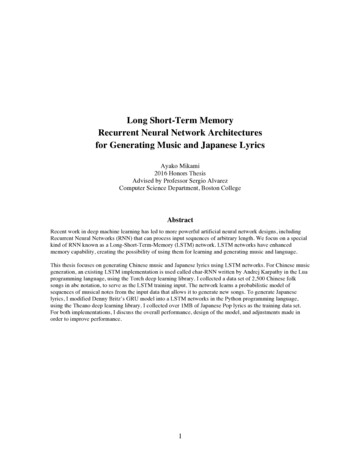
e17-6Muhammad I. Zafar et al.where W ðlÞ and bðlÞ represent the weight matrix and bias vector for the lth layer, respectively, and f is anactivation function. Activation functions enable the representation of complex functional mapping byintroducing nonlinearity in the composite functions. The training of a neural network is a process oflearning the weights and biases with the objective of fitting the training data.RNNs are architectures with internal memory (known as the hidden states), which make themparticularly suitable for sequential data such as time series, spatial sequences, and words in a text. TheRNN processes the sequence of inputs in a step-by-step manner while selectively passing the informationacross a sequence of steps encoded in a hidden state. At any given step i, the RNN operates on the currentinput vector (qi ) in the sequence and the hidden state hi 1 passed on from the previous step, to produce anupdated hidden state hi and an output yi . Figure 2 shows the schematic of a recurrent neural network.Multiple RNNs can be stacked over each other, as shown in Figure 3, to provide a deep RNN. Thefunctional mapping for an architecture with L layers of RNN stacked over each other can be expressed as:hihli ¼ f W lhh hli 1 þ W lqh hl 1,(2a)iyi ¼ W hy hLi ,(2b)where W lhh , W lqh , and W hy are the model parameters corresponding to the mapping from a previoushidden state to subsequent hidden state, from an input vector to a hidden state, and from a hidden state toan output vector, respectively. The model parameters (W lhh and W lqh ) have sequential invariance acrosseach layer, that is, the input vector and hidden state at each step along the sequence are processed by thesame parameters within a given layer of the RNN architecture. For the first layer, hl 1is equivalent to theiinput vector qi , while for subsequent layers, hl 1denotesthehiddenstatefromthepreviouslayer at theicurrent step. In this manner, a multilayer RNN transmits the information encoded in the hidden state to thenext step in the current layer and to the current step of the next layer by implementing Equation (2a). Forthe sake of brevity, the bias terms have not been mentioned in these equations.Figure 2. Schematic of the recurrent neural network (RNN) cell shown as a blue box on the left. Withineach RNN cell, the arrangement of the weight matrices is shown on the right. At any step i of the sequence,the RNN cell takes input qi and previous hidden state hi 1 , and provides updated hidden state hi andoutput yi .https://doi.org/10.1017/dce.2021.11 Published online by Cambridge University Press

Data-Centric Engineeringe17-7Figure 3. Sequences of input features and output for deep recurrent neural network (RNN) architecturehave been illustrated with respect to stations along the airfoil surface.Like deep feed-forward neural networks, deep RNNs can lead to more expressive models. However,the depth of an RNN can have multiple interpretations. In general, RNN architectures with multiple RNNlayers stacked over each other are considered deep RNNs, as shown in Figure 3. Such deep RNNarchitectures have multiple internal memories (hidden states), one in each RNN layer. RNN architectureswith multiple recurrent hidden states, stacked over each other, can model varying levels of dependencies(i.e., from short-term to long-term) in each hidden state (Hermans and Schrauwen, 2013). These stackedRNN architectures can still be considered shallow networks with limited expressivity, as all modelparameters (W hh , W qh , and W hy ) are generally represented by single linear layers. To allow for morecomplex functional representation, these single linear layers can be replaced by multiple nonlinear layers.Pascanu et al. (2014) has shown that introducing depth via multiple nonlinear layers to represent W hh ,W qh , and W hy can lead to better expressivity of the RNN model. For the transition modeling problemaddressed in this paper, multiple nonlinear layers are used within each RNN cell to express the complexphysical mapping between the input features and output, as shown in Figure 2. Such architecture resultedin better learning and predictive capability of the RNN model.The underlying physics of transition does not require long term memory, unlike natural languageprocessing for which more involved models like long short-term memory (LSTM) and transformers haveproved to be very effective. For the transition problem, keeping track of last one or two stations haveproved to be sufficient. In a study at the start of this research work, an informal investigation showed noadvantage of LSTMs over RNNs, despite their added complexity and higher training cost.With this perspective, the RNN model being proposed in this paper maps the sequential dependency ofmean boundary-layer flow properties as input features to instability growth rates corresponding to the Nfactor envelope as output features. Such input and output features, summarized in Table 1, have beentaken at a sequence of stations along the airfoil surface as shown in Figure 3. Mean boundary-layer flowproperties have been introduced in terms of the Reynolds number (Re θ ) based on the local momentumthickness of the boundary layer, the velocity boundary-layer profile (u), and its derivatives (du dy andd 2 u dy2 ). Zafar et al. (2020) proposed a convolutional neural network model that encodes the informationhttps://doi.org/10.1017/dce.2021.11 Published online by Cambridge University Press

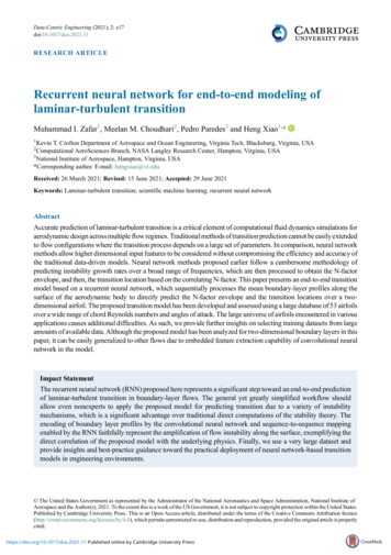
e17-8Muhammad I. Zafar et al.from boundary-layer profiles to a vector of latent features while accounting for the spatial patterns in theinput profiles (Michelén-Ströfer et al., 2018; Wu et al., 2018a). Such a treatment of boundary-layerprofiles allows the trained neural network models to generalize to all practical flows with differentinstability mechanisms (Paredes et al., 2020).The RNN model presented in this paper builds upon this idea and further combines CNN with RNN toaccount for nonlocal physics in both streamwise and wall-normal directions. This is shown in Figure 4.The hyperparameters of the proposed neural network have been empirically tuned to yield adequatecomplexity for learning all the required information, without causing an overfitting of the training data.After such hyperparameter tuning of the neural network model, early stopping was not required. With theboundary-layer profiles defined by using 41 equidistant points in the wall-normal direction, the CNNarchitecture contains 3 convolutional layers with 6, 8, and 4 channels, respectively, in those layers. Kernelsize of 3 1 has been used in each convolutional layer. Rectified linear unit (ReLU) is used as theactivation function. The CNN encodes the spatial information in the boundary-layer profiles along eachstation to a vector of latent features, Ψ. The results are not significantly sensitive to the number of latentfeatures in the vector Ψ. However, following a sensitivity study on the size of latent features, the number ofelements in Ψ has been set to 8. The latent features Ψ extracted from the boundary-layer profiles are thenTable 1. Input features and output for the RNN model.Feature/outputDescriptionq1q2Reynolds number based on edge velocity and momentumthicknessVelocity profile as a function of wall normal coordinate yq3First-order derivative of velocity profileq4Second-order derivative of velocity profiley1Slope of N-factor envelope, corresponding to local growth rateof the most amplified disturbance at that locationDefinitionRe θu j , j ¼ 1,2, , 41 du dy j , j ¼ 1, 2, ,41 d 2 u 2 , j ¼ 1, 2, ,41dyjdN env dsFigure 4. Proposed neural network for transition modeling. Convolutional neural network encodes theinformation from boundary-layer profiles (u,uy ,uyy ) into latent features (Ψ) at each station. RNNprocesses the input features (Re θ and Ψ) in sequential manner to predict the growth rate (dN ds) of theN-factor envelope.https://doi.org/10.1017/dce.2021.11 Published online by Cambridge University Press

Data-Centric Engineeringe17-9concatenated with Re θ at each station, which provides the sequential input features for the RNNarchitecture to predict the local growth rate of the most amplified instability mode, or equivalently, theslope (dN ds) of the N-factor envelope at a sequence of stations along the airfoilEach RNN cell surface. (Figure 2) consists of nonlinear mappings from the input to the hidden state W qh and from the hiddenstate to the output (W hy ), with each mapping involving two hidden layers with 72 neurons each. Therectified linear activation function (ReLU) is used to introduce nonlinearity in these layers. The hiddenstate is represented by a vector of length 9 and a linear layer is used for the mapping W hh between thehidden states. The RNN architecture consists of three RNN layers stacked over each other, withcorresponding three internal memories (hidden states), each representing varying level of dependency(short to long term) between the output at the current station and the input at the current as well as thepreceding stations.As the CNN architecture is intrinsically dependent on the shape of the training data, the architecture canbe tuned to different shapes of training data and the proposed model is expected to maintain its efficiencyand accuracy. Future work will explore the vector-cloud neural network Zhou et al. (2021) which can dealwith any number of arbitrarily arranged grid points across the boundary layer profiles. Since empiricaltuning of hyperparemeters provided good results, we did not undertake an extensive optimization of thewhole model. In a related unpublished work, more extensive hyperparameter optimization resulted inminor adjustments of the CNN architecture with comparable results.3. Database of Linear Amplification Characteristics for Airfoil Boundary LayersA large database of the linear stability characteristics of two-dimensional incompressible boundarylayer flows over a broad set of airfoils was generated for the training and evaluation of the proposedmodel. These boundary-layer flows can support the amplification of TS waves and the most amplifiedTS waves at any location along the airfoil correspond to two-dimensional disturbances (i.e., spanwisewavenumber β ¼ 0). This database documents the amplification characteristics of unstable TS wavesunder the quasiparallel, no-curvature approximation. A value of N tr ¼ 9 has been empirically found tocorrelate with the onset of laminar-turbulent transition in benign freestream disturbance environmentscharacteristic of external flows at flight altitudes. The airfoil contours were obtained from publicdomain sources, such as the UIUC Airfoil Coordinates Database (UIUC Applied Aerodynamics Group,2020). Linear stability characteristics for laminar boundary-layer flows were computed using acombination of potential flow solutions (Drela, 1989) and a boundary-layer solver (Wie, 1992). Thecomputational codes used are industry standard and have been used in number of research works overthe years. Inviscid computations using panel method have been performed with 721 points around theairfoil. For boundary layer solver, 300–400 grid points have been considered in wall normal directionusing a second order finite difference scheme. We note that the focus of this database is on transition dueto TS waves in attached boundary layers, and therefore, flows

RESEARCH ARTICLE Recurrent neural network for end-to-end modeling of laminar-turbulent transition Muhammad I. Zafar1, Meelan M. Choudhari2, Pedro Paredes3 and Heng Xiao1,* 1Kevin T. Crofton Department of Aerospace and Ocean Engineering, Virginia Tech, Blacksburg, Virginia, USA 2Computational AeroSciences Branch, NASA Langley Research Center, Hampton, Virginia, USA