Transcription
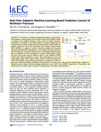
Articlepubs.acs.org/IECRCite This: Ind. Eng. Chem. Res. 2020, 59, 2275 2290Real-Time Adaptive Machine-Learning-Based Predictive Control ofNonlinear ProcessesZhe Wu,† David Rincon,† and Panagiotis D. Christofides*,†,‡†Department of Chemical and Biomolecular Engineering, University of California, Los Angeles, California 90095, United StatesDepartment of Electrical and Computer Engineering, University of California, Los Angeles, California 90095, United StatesDownloaded via UNIV OF CALIFORNIA LOS ANGELES on February 22, 2020 at 17:05:06 (UTC).See https://pubs.acs.org/sharingguidelines for options on how to legitimately share published articles.‡ABSTRACT: We present a machine learning-based predictive control schemethat integrates an online update of the recurrent neural network (RNN) modelsto capture process nonlinear dynamics in the presence of model uncertainty.Specifically, an ensemble of the RNN models are initially obtained for thenominal system, for which Lyapunov-based model predictive control (LMPC) isutilized to drive the state to the steady-state, and economic Lyapunov-basedMPC (LEMPC) is applied to achieve closed-loop stability and economicoptimality simultaneously. Subsequently, an event-trigger mechanism based onthe decreasing rate of Lyapunov function and an error-trigger mechanism thatrelies on prediction errors are developed for an online model update, in whichthe most recent process data are utilized to derive a new ensemble of RNNmodels with enhanced prediction accuracy. By incorporating the event anderror-triggered online RNN update within real-time machine learning-basedLMPC and LEMPC, process dynamic performance is improved in terms ofguaranteed closed-loop stability, optimality, and smoothness of control actions. The proposed methodology is applied to achemical process example with time-varying disturbances under LMPC and LEMPC, respectively, to demonstrate theeffectiveness of an online update of machine learning models in real-time control problems. INTRODUCTIONModeling large-scale, complex nonlinear processes has been along-lasting challenge in process systems engineering. Modelquality depends on many factors, including, but not limited toparameter estimation, model uncertainty, number of assumptions made in model development, dimensionality, modelstructure, and computational burden of solving the model inreal-time operations.1,2 Machine learning techniques have beensuccessfully applied to solve regression/modeling problemsbased on data sets from industrial process operation ornumerical simulations in process engineering, when a firstprinciples model is difficult to obtain. Among many machinelearning methods, recurrent neural networks (RNN), a class ofartificial neural network consisting of both feed-forward andfeedback connections layers,3 show promising potential for usein model-based control systems since they are capable ofmodeling nonlinear dynamical systems using time-series processdata. In refs 4 and 5 neural networks have been applied inindustrial control problems. In refs 6 8 machine learningtechniques have been applied to control chemical engineeringsystems. In ref 9 a comparison between feed-forward neuralnetworks and recurrent neural networks in nonlinear modelingand prediction has been discussed. Recently, RNN models havebeen incorporated in the design of model predictive control(MPC) systems to operate the system at its steady-state10,11while accounting for input and stability constraints. Additionally, based on the economic model predictive control (EMPC)that has been proposed to address process control problems 2019 American Chemical Societyaccounting for process dynamics (e.g., valve actuator dynamicsand actuator stiction compensation12,13) and dynamic economicoptimization, a new class of EMPC systems that takes advantageof RNN models to predict future states has been developed in ref14 to dynamically optimize process operating profit and achieveclosed-loop stability. Although pretrained machine learningmodels have demonstrated to be good replacements for firstprinciples models in model-based controllers, a potentialproblem for the real-time implementation of controllers inpractice is model uncertainty, which includes intrinsic andexogenous uncertaint.15,16Since in real life, processes models change in time due tovarying process parameters from external (e.g., aging equipment,disturbance, and new implemented technology in the process)and internal factors (e.g., fouling in the equipment), the machinelearning model that has been trained using the information frompast normal operations may not be able to correctly predictprocess states after disturbances appear. Some efforts have beenmade to circumvent model uncertainty using adaptive, robust,and event-triggered control within classical (first-principles)modeling and data-driven modeling techniques (e.g., neuralnetwork). For example, in the adaptive control area, aSpecial Issue: Christos Georgakis 5June 5, 2019July 15, 2019July 24, 2019July 24, 2019DOI: 10.1021/acs.iecr.9b03055Ind. Eng. Chem. Res. 2020, 59, 2275 2290
ArticleIndustrial & Engineering Chemistry Researchimplementation strategies of online RNN learning mechanismswithin LMPC and LEMPC, respectively, are presented withguaranteed closed-loop stability for both cases. In the lastsection, the proposed LMPC and LEMPC with the onlineupdate of the RNN models are applied to a nonlinear chemicalprocess example to demonstrate their effectiveness.methodology was proposed for high-dimensional nonlinearsystems using neural networks under a triangular structure in thecontrol inputs in which stability is guaranteed17. Similarly, thestability of an adaptive neural control system for two types ofmodel uncertainty of multi-input/multi-output nonlinearsystems is proven in block-triangular forms.1 From a robustcontrol point of view, an H controller was designed using arecurrent neural network for compensating parameter variationsand external disturbances.18 However, the above methodologieshave limitations. They are only applicable to systems in whichthe affected parameter is known a priori and a predefinedstructure is needed for the inputs and the states. Additionally, inrefs 19 22 the effects of model uncertainty were discussed, anddata-driven models were developed to account for processuncertainty.Considering the need to update process models as timeevolves, online learning of process models using most recentprocess data may provide a solution to deal with modeluncertainty. For example, in ref 23, a multistage online learningprocess was proposed using a hybrid neural network model for areal-time control of traffic signals to account for the variation oftraffic volume. In ref 24 the error-triggered model reidentification has been utilized to update the process model in EMPCwhen the error between predicted states and measured statesexceeds a threshold. It is noted that the event-triggeredmechanism is able to reduce the frequency of the online updateand adjustment of process models and control actions,25,26 andthus, improve applicability and efficiency of real-time control.For example, in ref 27 an event-based control was proposed toupdate the actuators only when a certain threshold is violated. Inref 26 an event-triggered mechanism was proposed to stabilizethe system with control actions being updated when a violationof a stability event is triggered. Additionally, the even-triggeredconcept has also been adopted in neural network-based controlto reduce the network source utilization.28,29 At this stage, theintegration of the online update of the RNN models with theproposed MPC and EMPC using an ensemble of RNN modelsin refs 10 and 14 remains an open issue.Motivated by the above, in this work, we propose real-timemachine learning-based MPC and EMPC schemes that triggeran online learning of the RNN models when a threshold isviolated due to unknown disturbances. Specifically, an ensembleof RNN models is initially obtained for the Lyapunov-basedMPC (LMPC) and Lyapunov-based EMPC (LEMPC) tostabilize the system under normal operation (i.e., withoutdisturbances). In the presence of time-varying disturbances, anevent-triggered mechanism based on the decreasing rate ofLyapunov function and an error-triggered mechanism based onthe prediction errors are developed to update RNN modelsduring the operation using the most recent process data. Closedloop stability analysis is performed for both LMPC and LEMPCwith the online RNN model update.The rest of this paper is organized as follows: in Preliminaries,the notations, the class of nonlinear systems considered, and thestabilizability assumptions are given. In the section “LyapunovBased MPC Using Ensemble of RNN Models”, the generalstructure of the recurrent neural network and the learningalgorithm are introduced. Then, a brief recap of the Lyapunovbased MPC and Lyapunov-based economic MPC using anensemble of RNN models are provided. In the section “EventTriggered On-Line Learning of RNNs”, the event-triggered anderror-triggered online RNN learning mechanisms are developed.In “Integration of On-Line Update of RNNs with MPC”, the PRELIMINARIESNotation. The notation · is used to denote the Euclideannorm of a vector. xT denotes the transpose of x. The notation V (x)Lf V(x) denotes the standard Lie derivative Lf V (x) x f (x)Set subtraction is denoted by “\”, that is, A\B {x Rn x A,x B}. denotes the set of positive integers. signifies thenull set. The function f(·) is of class *1 if it is continuouslydifferentiable in its domain. A continuous function α: [0, a) [0, ) is said to belong to class 2 if it is strictly increasing and iszero only when evaluated at zero.Class of Systems. The class of continuous-time nonlinearsystems considered is described by the following system of firstorder nonlinear ordinary differential equations:x ̇ F(x , u , w) f (x) g (x)u h(x)w , x(t0) x0(1)where x Rn is the state vector, u Rm is the manipulated inputvector, and w W is the disturbance vector with W {w Rq w wm, wm 0}. The control actions are constrained by u Um {umin ui umaxii , i 1, ., m} R . f(·), g(·), and h(·) aresufficiently smooth vector and matrix functions of dimensions n 1, n m, and n q, respectively. Throughout the manuscript,we assume that the initial time t0 is zero (t0 0), and f(0) 0such that the origin is a steady-state of the nominal (i.e., w(t) 0) system of eq 1 (i.e., (x*s , u*s ) (0,0), where x*s and u*srepresent the steady-state state and input vectors, respectively).Stabilization via Control Lyapunov Function. Toguarantee that the closed-loop system can be stabilized, astabilizing control law u Φ(x) U that renders the origin ofthe nominal system of eq 1 (i.e., w(t) 0) exponentially stable isassumed to exist. Following converse theorems,30 there exists a*1 Control Lyapunov function V(x) such that the followinginequalities hold for all x in an open neighborhood D around theorigin:c1 x 2 V (x) c 2 x 2 ,(2a) V (x)F(x , Φ(x), 0) c3 x 2 , x(2b) V (x) c4 x x(2c)where c1, c2, c3, and c4 are positive constants. F(x, u, w) representsthe nonlinear system of eq 1. The universal Sontag control law31is a candidate controller for u Φ(x).We first characterize a region where the time-derivative of V isrendered negative under the controller u Φ(x) U as follows:ϕu {x Rn V̇ (x) Lf V Lg Vu k x 2 ,u Φ(x) U} {0}(3)where k is a positive real number. Then a level set of theLyapunov function inside ϕu is used as the closed-loop stabilityregion Ωρ for the nonlinear system of eq 1 as follows: Ωρ {x 2276DOI: 10.1021/acs.iecr.9b03055Ind. Eng. Chem. Res. 2020, 59, 2275 2290
ArticleIndustrial & Engineering Chemistry Researchϕu V(x) ρ}, where ρ 0 and Ωρ ϕu. From the Lipschitzproperty of F(x, u, w) and the bounds on u and w, it follows thatthere exist positive constants M, Lx, Lw, Lx′, Lw′ such that thefollowing inequalities hold for all x, x ′ D, u U, and w W: F(x , u , w) M(4a) F(x , u , w) F(x′, u , 0) Lx x x′ Lw w (4b)that is updated using the real-time data of closed-loop statetrajectories and control actions, where NT is the total number ofRNN models obtained. We assume that a set of stabilizingfeedback controllers u Φinn(x) U that can render the origin ofthe RNN models Finn(x, u), i 1,2, ., NT of eq 5 exponentiallystable in an open neighborhood D̂ around the origin exists.Therefore, there exists a *1 Control Lyapunov function V̂ (x)such that the following inequalities hold for all x in D̂ : V (x′) V (x)F(x′, u , 0)F(x , u , w) x x Lx′ x x′ Lw′ w (4c)LYAPUNOV-BASED MPC USING ENSEMBLE RNNMODELSIn this section, the structure of a recurrent neural network(RNN) model and the formulation of the Lyapunov-based MPC(LMPC) and Lyapunov-based economic MPC (LEMPC) usingthe RNN model ensemble to predict future states are presented.Specifically, an RNN model is first developed to approximate thenonlinear dynamics of the system of eq 1 in the operating regionΩρ using data from extensive open-loop simulations. Subsequently, LMPC and LEMPC are developed using an ensembleof RNN models to derive closed-loop stability for the nonlinearsystem of eq 1.Recurrent Neural Network. The recurrent neural networkmodel is developed with the following form:x ̂ ̇ Fnn(x ̂ , u) Ax ̂ ΘTy(7a) V̂ (x) iFnn(x , Φinn(x)) c3̂ i x 2 x(7b) V̂ (x) c4î x x(7c)where ĉi1, ĉi2, ĉi3, and ĉi4 are positive constants, i 1, 2, ., NT. Forthe sake of simplicity, we will use symbols without thesuperscript of i for all the RNN models and controllers thatsatisfy eq 7 in the following texts. Similar to the characterizationmethod of the closed-loop stability region Ωρ for the nonlinearsystem of eq 1, we first characterize a regionϕû {x Rn V̂ ̇ (x) c3̂ x 2 , u Φmn(x) U} {0}from which the origin of the RNN model of eq 5 can be renderedexponentially stable under the controller u Φnn(x) U.The closed-loop stability region for the RNN model of eq 5 isdefined as a level set of Lyapunov functions inside ϕ̂ u: Ωρ̂ {x ϕ̂ u V̂ (x) ρ̂}, where ρ̂ 0. It is noted that Ωρ̂ Ωρ since thedata set for developing the RNN model of eq 5 is generated fromopen-loop simulations for x Ωρ and u U. Additionally, thereexist positive constants Mnn and Lnn such that the followinginequalities hold for all x, x ′ Ωρ̂ and u U:(5)where x̂ Rn is the RNN state vector and u Rm is themanipulated input vector. y [y1, ., yn, yn 1, ., ym n] [σ(x̂1),., σ(x̂n), u1, ., um] Rn m is a vector of both the network state x̂and the input u, where σ(·) is the nonlinear activation function(e.g., a sigmoid function σ(x) 1/(1 e x)). A is a diagonalcoefficient matrix; that is, A diag{ a1, ., an} Rn n, ai 0,and Θ [θ1, ., θn] R(m n) n with θi bi[wi1, ., wi(m n)],where bi, i 1, ., n are constants. wij is the weight connecting thejth input to the ith neuron where i 1, ., n and j 1, ., (m n).Throughout the manuscript, we use x to represent the state ofthe actual nonlinear system of eq 1 and use x̂ for the state of theRNN model of eq 5.The RNN model is trained following the learning algorithm inref 14 to obtain the optimal weight vector θ*i by minimizing thefollowing loss function:N looo dT oθi* arg min m F(x,u,0) ax θy i kki ki k }ooo θi θmonk 1 c1̂ i x 2 V̂ (x) c 2̂ i x 2 Fnn(x , u) Mnn(8a) V̂ (x′) V̂ (x)Fnn(x′, u) Lnn x x′ Fnn(x , u) x x(8b)Consider that there exists a bounded modeling error betweenthe nominal system of eq 1 and the RNN model of eq 5 (i.e., ν F(x, u,0) Fnn(x, u) νm, νm 0), the following propositiondemonstrates that the feedback controller u Φnn(x) U is ableto stabilize the nominal system of eq 1 if the modeling error issufficiently small.Proposition 1 (ref 10). Under the assumption that the originof the closed-loop RNN system of eq 5 is rendered exponentiallystable under the controller u Φnn(x) U for all x Ωρ̂, if thereexists a positive real number γ ĉ3/ĉ4 that constrains themodeling error ν F(x, u,0) Fnn(x, u) γ x νm for all x Ωρ̂ and u U, then the origin of the nominal closed-loopsystem of eq 1 under u Φnn(x) U is also exponentially stablefor all x Ωρ̂.LMPC Using an Ensemble of RNN Models. Theformulation of the LMPC using an ensemble of RNN modelsis given as follows:10(6)where Nd is the number of data samples used for training. Tofurther improve the prediction accuracy of the RNN model,ensemble learning that combines multiple machine learningmodels is utilized to obtain the final predicted results.Specifically, following the method in ref 14, k different RNNmodels Fnn, i(x, u), i 1, ., k, are trained via a k-fold crossvalidation to approximate the same nonlinear system. Theaveraged results are calculated as the final output of theensemble of multiple RNN models.Lyapunov-Based Control Using an Ensemble of RNNModels. In this work, the RNN model of eq 5 is updated tocapture nonlinear dynamics of the nonlinear system of eq 1subject to time-varying bounded disturbances (i.e., w(t) wm).Finn(x, u) is used to denote the ith RNN model (i 1, 2, ., NT) u S(Δ) ttk N1 min2277kL(x(̃ t ), u(t )) dt(9a)DOI: 10.1021/acs.iecr.9b03055Ind. Eng. Chem. Res. 2020, 59, 2275 2290
ArticleIndustrial & Engineering Chemistry Researchs.t.x(̃̇ t ) 1Neultimately converges to Ωρmin for the nominal closed-loop systemof eq 1.Proof. The proof of Theorem 1 can be found in ref 10.LEMPC Using an Ensemble of RNN Models. TheLyapunov-based economic MPC (LEMPC) using an ensembleof RNN models is developed to dynamically optimize processeconomic benefits while maintaining the closed-loop state in thestability region for all times.14 The LEMPC is represented by thefollowing optimization problem:Ne Fnn,j(x(̃ t ), u(t ))(9b)j 1u(t ) U , t [tk , tk N )(9c)x(̃ tk) x(tk)(9d)V̂ ̇ (x(tk), u) V̂ ̇ (x(tk), Φnn(x(tk)),if x(tk) Ω ρ \Ω̂ρnn(9e)V̂ (x(̃ t )) ρnn , t [tk , tk N ),if x(tk) Ω ρnn u S(Δ) twhere x̃ is the predicted state trajectory, S(Δ) is the set ofpiecewise constant functions with period Δ, N is the number ofsampling periods in the prediction horizon, and Ne is the numberof regression models used for prediction. V̂ ̇ (x , u) is used tos.t. V̂ (x)represent x (Fnn(x , u)). The optimal input trajectorycomputed by the LMPC is denoted by u*(t), which is calculatedover the entire prediction horizon t [tk, tk N). The controlaction computed for the first sampling period of the predictionhorizon u*(tk) is sent by the LMPC to be applied over the firstsampling period, and the LMPC is resolved at the next samplingtime.In the optimization problem of eq 9, the objective function ofeq. 9a is the integral of L(x̃(t), u(t)) over the prediction horizon.The constraint of eq 9b is the ensemble of RNN models of eq 5(i.e., Fnn, j, j 1, ., Ne) that is used to predict the states of theclosed-loop system. eqation 9c defines the input constraintsapplied over the entire prediction horizon. eqation 9d definesthe initial condition x̃(tk) of eq 9b, which is the statemeasurement at t tk. The constraint of eq 9e forces theclosed-loop state to move toward the origin if x(tk) Ωρ̂\Ωρnn.However, if x(tk) enters Ωρnn, the states predicted by the RNNmodel of eq 9b will be maintained in Ωρnn for the entireprediction horizon.Based on the LMPC of eq 9, the following theorem isestablished to demonstrate that the LMPC optimizationproblem can be solved with recursive feasibility, and closedloop stability of the nonlinear system of eq 1 is guaranteed underthe sample-and-hold implementation of the optimal controlactions calculated by LMPC.Theorem 1. Consider the nominal closed-loop system of eq 1(i.e., w(t) 0) under the LMPC of eq 9 based on the RNNmodel of eq 5 that satisfies γ ĉ3/ĉ4 and the controller Φnn(x)that satisfies eq 7. Let Δ 0, εw 0, and ρ̂ ρmin ρnn ρs satisfythe following inequalities:c̃ 3 ρs Lx′M Δ εwc 2̂(10)ρmin ρnn c4̂ ρ ̂c1̂fw (Δ) κ(fw (Δ))2where c̃3 ĉ3 ĉ4γ 0 and fw (t ) νm Lxt(eLxx(̃̇ t ) le(x(̃ t ), u(t )) dt(12a)k1NeNe Fnn,j(x(̃ t ), u(t ))(12b)j 1u(t ) U , t [tk , tk N )(12c)x(̃ tk) x(tk)(12d)V̂ (x(̃ t )) ρê , t [tk , tk N ),if x(tk) Ω ρêV̂ ̇ (x(tk), u) V̂ ̇ (x(tk), Φnn(x(tk)),(12e)if x(tk) Ω ρ \Ω̂ρê(12f)where the notations of eq 12 follow those of eq 9. Theoptimization problem of eq 12 optimizes the time integral of thestage cost function le(x̃(t), u(t)) of eq 12a over the predictionhorizon. The prediction model of eq 12b and the initialcondition of eq 12d are the same as those in the LMPC of eq 9.The constraint of eq 12e maintains the predicted closed-loopstates in Ωρ̂e over the prediction horizon if x(tk) is inside Ωρ̂e.However, if x(tk) enters Ωρ̂\Ωρ̂e, the contractive constraint of eq12f drives the state toward the origin for the next samplingperiod such that the state will eventually enter Ωρ̂e within finitesampling periods.Theorem 2. Consider the nominal closed-loop system of eq 1under the LEMPC of eq 12 based on the controller Φnn(x) thatsatisfies eq 7. Let Δ 0, εw 0, and ρ̂ ρ̂e 0 satisfy eq 10 andthe following inequality:ρê ρ ̂ c4̂ ρ ̂c1̂fw (Δ) κ(fw (Δ))2(13)Then, for any x0 Ωρ̂, there always exists a feasible solution forthe optimization problem of eq 12, and the closed-loop statex(t) is bounded in the closed-loop stability region Ωρ̂, t 0.Proof. The proof of Theorem 2 can be found in ref 14.Remark 1. The RNN model is used in this work because it isable to model a continuous nonlinear dynamical system of eq 1,while a simpler artificial neural network (i.e., feed-forward neuralnetwork) is typically used to describe a steady-state relationship.Since LMPC and LEMPC rely on a continuous dynamic processmodel to predict future states, the RNN model is preferred inthis study.Remark 2. In this work, the RNN models are developed toreplace the first-principles models used in MPC. It is noted thatneural networks can also be applied to approximate the entireMPC.32 The differences between the RNN model that replacesthe first-principle model and the artificial neural network(ANN) that approximates the entire MPC are as follows: (1)the data set for RNN models are obtained from extensive open-andρnn max{V̂ (x(̂ t Δ)) x(̂ t ) Ω ρs , u U}tk N1 max(9f)(11a)(11b) 1). Then, givenany initial state x0 Ωρ̂, there always exists a feasible solution forthe optimization problem of eq 9. Additionally, it is guaranteedthat under the LMPC of eq 9, x(t) Ωρ̂, t 0, and x(t)2278DOI: 10.1021/acs.iecr.9b03055Ind. Eng. Chem. Res. 2020, 59, 2275 2290
ArticleIndustrial & Engineering Chemistry Researchwhere εw 0 and ρs satisfy eq10 and eq 11 in Theorem 1, thenthere exists a positive constant τ* such that the minimalinterevent time Tk rk 1 rk τ*.Proof. Since the controller u Φnn(x) U is implemented ina sample-and-hold fashion, given x(tk) x̂(tk) Ωρ̂\Ωρs, we firstderive the time-derivative of V̂ (x) for the nonlinear system of eq1 (i.e., ẋ F(x, u, w)) in the presence of bounded disturbances(i.e., w wm) over t [tk, tk 1) as follows:loop simulations that capture process dynamics in the operatingregion, while the data set for the ANN that replaces MPC isdeveloped based on closed-loop simulations under MPC. (2)Since the RNN model is derived to replace the first-principlesmodel in the manuscript, the optimization problem of MPC stillneeds to be explicitly defined (e.g., objective function andconstraints) and solved online. However, if the ANN is obtainedto replace the entire MPC, the optimization problem of MPC isreplaced by an input output function described by an ANN.Additionally, it is noted that the obtained ANN may only workfor the same MPC problem that is used to generate the closedloop data set. Any modifications to the objective function or theconstraints may lead to regeneration of the data set andretraining of neural networks. Therefore, it is more convenientto develop and incorporate RNN models in MPC due to itseasily accessible open-loop data set and the freedom to makemodifications in MPC formulation. However, if the computational efficiency is of significant importance, ANNs that replacethe entire MPC can be regarded as a good solution to savingcomputation time and computing control actions for the closedloop system. V̂ (x(t ))F(x(t ), Φnn(x(tk)), w(t )) x V̂ (x(tk))F(x(tk), Φnn(x(tk)), w(tk)) x V̂ (x(t ))F(x(t ), Φnn(x(tk)), w(t )) x V̂ (x(tk))F(x(tk), Φnn(x(tk)), w(tk)) xV̂ ̇ (x(t )) The first term V̂ (x(tk))F(x(tk), Φnn(x(tk)), w(tk)) xEVENT-TRIGGERED ONLINE LEARNING OF RNNSIn this section, the LMPC of eq 9 and the LEMPC of eq 12 areapplied to the nonlinear system of eq 1 subject to boundeddisturbances (i.e., w(t) wm). Unlike the stability analysisperformed for sufficiently small bounded disturbances in refs 10and 14, in this work, we consider the case in which disturbancescannot be fully eliminated by the sample-and-hold implementation of LMPC and therefore, may render the closed-loop systemunstable. To mitigate the impact of disturbances, RNN modelsare updated via online learning to capture the nonlineardynamics of the system of eq 1 accounting for disturbancesw(t). In the following subsections, the triggering mechanisms forupdating RNN models are introduced.Event-Triggering Mechanism. In ref 33 event-triggeredand self-triggered control systems were introduced to deriveclosed-loop stability for the system under the sample-and-holdimplementation of a controller. Specifically, the event-triggeredcontrol system triggers an update of control actions if atriggering condition based on state measurements is violated,while in a self-triggered control system, the next update time canbe obtained via predictions. In our work, an event-triggeredonline RNN learning is incorporated in the LMPC of eq 9 andthe LEMPC of eq 12 to improve RNN prediction accuracy usingpreviously received data of closed-loop states in the presence ofbounded disturbances. The following theorem is established todemonstrate that if the online update of RNN is triggered by theviolation of eq 14, the minimal interevent time Tk rk 1 rk isbounded from below, where rk represents the kth violation of eq14, k .Theorem 3. Consider the nonlinear system ẋ F(x, u, w) ofeq 1 in the presence of bounded disturbances w(t) wm, andthe RNN model x̂̇ Fnn(x̂, u) of eq 5 that has been updated at t tk rk to approximate the dynamic behavior of the system of eq 1before t tk with a sufficiently small modeling error ν γ x , γ ĉ3/ĉ4. If the stabilizing controller u Φnn(x) U is implementedin a sample-and-hold fashion (i.e., u(t) Φnn(x̂(tk)), t [tk,tk 1), where tk 1 tk Δ and Δ is the sampling period), andthe k 1th update of the RNN model is triggered at t rk 1 bythe violation of the following inequality for all x Ωρ̂\Ωρs:V (x(t )) V (x(tk)) εw(t tk), t [tk , tk 1)(15)in the above equation can be further expanded as follows: V̂ (x(tk))F(x(tk), Φnn(x(tk)), w(tk)) x V̂ (x(tk)) (Fnn(x , Φnn(x(tk))) x F(x , Φnn(x(tk)), w(tk)) Fnn(x , Φnn(x(tk)))) c3̂ x(tk) 2 c4̂ x(tk) (F(x(tk), Φnn(x(tk)), w(tk)) Fnn(x(tk), Φnn(x(tk)))) c3̂ x(tk) 2 c4̂ γ x(tk) 2 c3̃ x(tk) 2(16)where c̃3 ĉ3 ĉ4γ 0 is a positive real number that has beendefined in Theorem 1. Specifically, the inequalities in eq 16 arederived from the fact that V̂ (x(t ))Fnn(x(t ), Φnn(x)) c3̂ x(t ) 2 xholds for all x Ωρ̂\Ωρs, and the RNN model x̂̇ Fnn(x̂, u) iswell-trained at t tk such that the modeling error ν F(x, u, w) Fnn(x̂, u) , t [0, tk] is constrained by ν γ x . On the basisof eq16 and eq 4, the time-derivative of V̂ in eq 15 can besimplified as follows:V̂ ̇ (x(t )) c3̃ x(tk) 2 V̂ (x(t ))F(x(t ), Φnn(x(tk)), w(t )) x V̂ (x(tk))F(x(tk), Φnn(x(tk)), w(tk)) x c3̃ x(tk) 2 Lx′ x(t ) x(tk) Lw′ w(t ) w(tk) (17)Let p(t) V̂ (x(t)) and q(t) Ṽ (x(t)) V̂ (x(tk)) εw(t tk). Itis readily shown that p(t) and q(t) are *1 functions and p(tk) q(tk) V̂ (x(tk)) holds. It follows that q(̇ tk) Ṽ̇ (x(tk)) εw .(14)2279DOI: 10.1021/acs.iecr.9b03055Ind. Eng. Chem. Res. 2020, 59, 2275 2290
ArticleIndustrial & Engineering Chemistry ResearchAdditionally, using eq 2 and eq 17, ṗ(tk) is bounded by thefollowing inequality:The following proposition is developed to demonstrate that ifthe RNN model update is triggered within a certain samplingperiod, yet the control actions remain unchanged till the end ofthis sampling period, closed-loop stability is still guaranteed inthe sense that the closed-loop state moves toward the originwithin one sampling period for all x Ωρ̂\Ωρw, where ρw {V̂ (x) V̂ ̇ (x) ĉ x 2 2L′ w , u Φ (x) U}.maxp ̇(tk) V̂ ̇ (x(tk)) c3̃ x(tk) 2 Lx′ x(tk) x(tk) Lw′ w(tk) w(tk) c̃ 3 V̂ (x(tk))c 2̂x Ωρ̂3w mnnAdditionally, ρw is designed such that if the current state is insideΩρw, it will not leave Ωρ̂ within one sampling period.Proposition 2. Consider the system of eq 1 with boundeddisturbances (i.e., w(t) wm) under the sample-and-holdimplementation of the controller u Φnn(x) U. Let ρ̂ ρw 0and Δ satisfy eq 10 and the following inequality:(18)Therefore, it is derived that ṗ(tk) q̇(tk) for all x(tk) Ωρ̂\Ωρsc̃since εw is chosen to satisfy eq 10 (i.e., c3̂ ρs Lx′M Δ εw ).2Following the Lemma in ref 26, it is shown that the minimalinterevent time Tk satisfies Tk τ*, where τ* is the smallestpositive solution to the equation p(t) q(t), due to thecontinuity properties of p, q, ṗ, q̇. This completes the proof ofTheorem 3.Remark 3. Theorem 3 demonstrates that the existence of anonzero minimal interevent time Tk is guaranteed for thenonlinear system of eq 1 subject to the triggering condition of eq14. This implies that the above sample-a
techniques have been applied to control chemical engineering systems. In ref 9 a comparison between feed-forward neural networks and recurrent neural networks in nonlinear modeling ve been incorporated in the design of model predictive control (MPC) systems to operate the system at its steady .
