Transcription
HindawiJournal of Applied MathematicsVolume 2021, Article ID 8003952, 11 pageshttps://doi.org/10.1155/2021/8003952Research ArticleHierarchical Bayesian Spatio-Temporal Modeling forPM10 PredictionEsam Mahdi , Sana Alshamari , Maryam Khashabi , and Alya AlkorbiDepartment of Mathematics, Statistics and Physics, Qatar University, Doha, QatarCorrespondence should be addressed to Esam Mahdi; emahdi@qu.edu.qaReceived 30 May 2021; Revised 29 July 2021; Accepted 23 August 2021; Published 13 September 2021Academic Editor: Wei-Chiang HongCopyright 2021 Esam Mahdi et al. This is an open access article distributed under the Creative Commons Attribution License,which permits unrestricted use, distribution, and reproduction in any medium, provided the original work is properly cited. Thepublication of this article was funded by Qatar National Library.Over the past few years, hierarchical Bayesian models have been extensively used for modeling the joint spatial and temporaldependence of big spatio-temporal data which commonly involves a large number of missing observations. This articlerepresented, assessed, and compared some recently proposed Bayesian and non-Bayesian models for predicting the dailyaverage particulate matter with a diameter of less than 10 (PM10) measured in Qatar during the years 2016–2019. Thedisaggregating technique with a Markov chain Monte Carlo method with Gibbs sampler are used to handle the missing data.Based on the obtained results, we conclude that the Gaussian predictive processes with autoregressive terms of the latentunderlying space-time process model is the best, compared with the Bayesian Gaussian processes and non-Bayesiangeneralized additive models.1. IntroductionMany of the environmental data contain different scales ofvariability over space and time. For example, scientists fromenvironmental and public health sciences are typically interested in modeling the evolving process of the air pollutionduring the time over specified locations. Such a stochasticprocess is often high-dimensional, large, and complicatedwith nonstationary structures, so the traditional statisticalmethods are hampered by the need of advanced statisticaltechniques to specify the spatio-temporal dependency. Thiscan be quite practical with modern computers with highlevel computational programming. The spatio-temporalmodeling of PM10 and PM2:5 (particulate matter with diameters of less than 10 and 2.5 micrometers, respectively) is rapidly becoming an important component of most air qualitystudies [1–3]. Particulate matter (also called particle pollution) is a mixture of solid particles and liquid droplets foundin the air as a result of dust, soot, dirt, smoke caused by roadtransportation, and complex chemical reactions in the atmosphere such as sulfur dioxide and nitrogen oxides. Exposureto particle pollution is a public health hazard and can causeacute and chronic heart and lung diseases [4]. The largerthe values of particulate matters (PM) are, the more harmon short and long terms of public health is. World HealthOrganization’s (WHO) air quality guidelines recommendthat the annual and 24-hour mean concentrations shouldnot, respectively, exceed 20 and 50 microgram per cubicmetre (μg/m3) for PM10, and 10 and 25 μg/m3 for PM2.5.Countries with fast-developed infrastructure such as Qatarusually suffer from relatively high levels of PM air pollutant.In this regard, the WHO classified the air quality in Qatar aspoor and unsafe. In this paper, we focus our attention onmodeling the PM10 in Qatar because the PM2.5 data is inaccessible. The most recent data indicates that country’s annualaverage 24 hr PM10 concentration levels were ranged from126.69 μg/m3 to 184.55 μg/m3, which exceeds the recommended maximum of 50 μg/m3 [4–6].Several authors have developed spatio-temporal modelsfor analyzing the ambient of air pollution. Research in thisfield is back in dates to Cressie [7] and Goodall and Mardia[8]. Cressie et al. [9] compared the performance of Markovrandom field with the familiar geestatistical approach in prediction the PM10 concentrations around the city of
2Pittsburgh, United States of America. The authors did notmodel the joint temporal and spatial structure of observations. They first modeled the purely spatial structure ofobservations for one particular day, then they incorporatedthe temporal component in their final statistical modeling.Sun et al. [10] developed a spatial forecasting distributionfor unmeasured daily log PM10 average concentration givenfrom ten locations in Vancouver, Canada. At each monitoring site, Sun et al. [10] showed that the autoregressive modelof order one (AR(1)) described quite well the daily log PM10average values. The authors did not consider the Bayesianmodels in their approach. Golam Kibria et al. [11] proposeda multivariate spatial prediction methodology in a Bayesianapproach that is suited for spatio-temporal data observedat a small set of ambient monitoring stations at successivetime points. They demonstrated the usefulness of theirapproach by mapping PM2.5 at monitoring sites with different start-up times in the city of Philadelphia, USA. GolamKibria et al. [11] did not compare the performance of theirmodel with other non-Bayesian models that are commonlyused in literature. Shaddick and Wakefield [12] and Sahuand Mardia [13] used short-term spatio-temporal predictiveanalysis for modeling the PM2.5 and PM10 concentrationlevels. Zidek et al. [3] presented predictive distributions onnonmonitored PM10 values in Vancouver, Canada. Smithet al. [14] proposed a spatio-temporal model to predict theweekly averages of particulate matter concentrations withinthree southeastern states in the USA. Sahu et al. [15] modeled the PM2.5 by combining the rural background and theurban areas into one process. Cocchi et al. [1] developed ahierarchical Bayesian model for the daily average PM10values. Pollice and Lasinio [2] developed a Bayesian-basedkriging method for estimating the daily average PM10 concentration levels. Wikle et al. [16] provided an excellentreview of classical and Bayesian approaches for analyzingspatio-temporal data. Although Taylor et al. [6], Ahmadiet al. [5], and others have studied the relationship betweensome environmental conditions and particulate matter levelsassessing the air quality based on particulate matter levels indifferent locations in Qatar, they did not study the spatiotemporal variability of PM10. The main objective of thisresearch is to develop space-time models for daily PM10 airpollution levels in Qatar for the four years, 2016-2019 comparing the hierarchical Bayesian approach with other spatiotemporal recent methods. We develop spatial interpolationand forecasting model using iterative Markov chain MonteCarlo (MCMC) computation setup which is an effectivemethod for modeling a data with large number of missingvalues [17]. To the best of our knowledge, this will be the firststudy in Qatar, and we hope that this research will be helpfulto protect the environment and public health in Qatar.The rest of this article is organized as follows: Section 2provides a brief review of two-stage hierarchical Bayesianmodels that have been used for modeling spatio-temporaldata. A numerical example is given in Section 3 to demonstrate that the Bayesian approach accurately predicts thedaily average PM10 values with a large number of missingvalues comparing with non-Bayesian models. Finally, a conclusion is given in Section 4.Journal of Applied Mathematics2. Hierarchical Spatio-Temporal ModelWhen data is collected at different points in space and time,we should use a model that can, simultaneously, describe thedependency structure coming from the three sources of variations: time variation, space variation, and joint variabilitybetween time and space. Such a model is called a spacetime model (or spatio-temporal model, where spatio refersto space and temporal refers to time).In this article, we develop hierarchical models to predict the daily PM10 concentration levels which vary overtime and locations. The PM10 concentration levels do notoften follow the normal distribution. Thus, we usually modelthese values on the square-root scale or we use the logtransformation to stabilize the variance and enforce normality and to stabilize the variance [18]. We consider the squareroot scale to alleviate the departure from normality in ourresearch data.Let ℓ and t denote the two units of time where ℓ 1, , rrepresents the longer unit (e.g., year), and t 1, , T ℓ represents the shorter unit (e.g., day). Let Z ℓ ðs, tÞ denote theobserved value of the PM10 concentration, after any necessary transformation, at a given location s and over a givendiscrete time t. We assume that the spatial location s is atwo-dimensional vector describing the latitude-longitude(or equivalently northing and easting coordinates), and thetime unit is typically hour, day, month, or year. We alsoassume that the Z ℓ ðs, tÞ is observed at n monitoring sitesdenoted by si , i 1, , n and at time points denoted bytwo indices ℓ and t so that the total number of observationsis denoted by N n rℓ 1 T ℓ . In this article, we denote all themissing data by z , whereas all the observed data will bedenoted by z.The first stage of the hierarchy assumes that the observedvalues Zℓt , where Zℓt ðZ ℓ ðs1 , tÞ, ,Z ℓ ðsn , tÞÞ ′ , can bedecomposed into a true (latent) spatio-temporal processYℓt ðY ℓ ðs1 , tÞ, ,Y ℓ ðsn , tÞÞ ′ with an error term εℓt ðεℓ ðs1 , tÞ, ,εℓ ðsn , tÞÞ ′ . More specifically, the data (or measurement error) model in the first stage of the hierarchy isZℓt Yℓt εℓt , ℓ 1, , r, t 1, , T ℓ :ð1ÞThe error term εℓt is assumed to be a Gaussian whitenoise process with mean zero and constant variance σ2ε ,which is often called the nugget effect absorbing microscalevariability.The second stage assumes that the true process Yℓt has asystematic mean μℓt and a spatio-temporal error term. Themean can be modeled based on the past values of the unobserved variable or/and based on some relevant covariates.Typically, Yℓt can be specified in the following formula:Yℓt μℓt ηℓt ,ð2Þwhere ηℓt ðηℓ ðs1 , tÞ, ,ηℓ ðsn , tÞÞ ′ is an spatio-temporalresidual random intercept assumed to follow N ð0, CÞ, whereC σ2η H η , σ2η is the site invariant spatial variance, and H η isthe spatial correlation matrix. In this article, we consider
Journal of Applied Mathematics3four modelings for fηℓt g. The first one assumes that the random effects, ηℓ ðsi , tÞ 0, for all locations si and times t. Thisimplies that the model in (1)–(2) will be the simple regression model. The other models for fηℓt g are assumed to beGaussian process, independent over the time, which is specified in Sections 2.1, 2.2, 2.3, and 2.4.2.1. Matérn Spatio-Temporal Covariance Function. Forspatio-temporal modeling, we usually assume that the random effects process is a weakly stationary Gaussian with azero mean and a valid isotropic covariance function. A validcovariance function implied that the covariance matrix ispositive definite, and isotropic means that the separationvector between the two locations only depends on the distance and not on the direction. The class of the spatiotemporal covariance functions can be separable, productsum, metric, and sum-metric [19]. In this paper, we usethe separable covariance model which is simply the productof the pure spatial covariance function, Cs ðhÞ, by the puretemporal one, C t ðuÞ, given byC ðh, uÞ Cs ðhÞC t ðuÞ, C wðs, t Þ, w s ′ , t pffiffiffi κ2 κ s s ′ ϕ K κ κ 12 ΓðκÞ pffiffiffi pffiffiffi 2 κ 2 κ s s ′ ϕ ϕ , ϕ 0, κ 1,N1 r ℓlog σ2ε 2 ðZℓt Yℓt Þ ′ ðZℓt Yℓt Þ22σε ℓ 1 t 1T 1 r1 r ℓ T ℓ log σ2η H η 2 2 ℓ 12ση ℓ 1 t 1ð5Þð6Þ ðYℓt Xℓt βÞ ′ H 1η ðYℓt X ℓt βÞ log pðθÞ,where pðθÞ is the prior distribution [21] and we refer thereaders to Bakar and Sahu ([21], Appendix A) to obtain theGibbs sampling using the full conditional distributions of θ.2.3. Autoregressive Model Specification. The autoregressiveprocess (AR) model in Equations (1) and (2) can be writtenin the hierarchical form (e.g., [18] model) as follows:Yℓt ρYℓt 1 Xℓt β ηℓt ,ð4Þ2.2. Gaussian Process Model Specification. Consider μℓt Xℓt β in (2), where ℓ 1, , r, t 1, , T ℓ , Xℓt is the n ðk 1Þ design matrix of spatially and temporally varying k-covariates and β ðβ0 , β1 , ,βk Þ ′ is the k 1-dimensionalvector of regression coefficients. Thus, the Gaussian process(GP) two-stage model can be written asYℓt Xℓt β ηℓt :T Zℓt Yℓt εℓt ,where K κ ð·Þ is the modified Bessel function of second kind oforder κ which is a parameter controlling the smoothness ofthe realized random field [20], ΓðκÞ is the standard gammafunction, and ϕ is a parameter which controls the decay ratein the correlation as the distance h increases. Popular specialcases of Matérn model are (i) κ 0:5 leads to exponentialcovariance function CðhÞ σ2η exp ð ϕhÞ and (ii) Gaussianmodel, CðhÞ σ2η exp ð ϕ2 h2 Þ when κ .Zℓt Yℓt εℓt ,log pðθ, Y, z zÞð3Þwhere h ks s ′ k is the separating spatial distance, andu jt t ′ j is the temporal distance for any pair of pointsðs, tÞ ðs ′ , t ′ Þ in the spatial and temporal study domain.The Matérn family provides a general choice of covariance functions. For each time t, the Matérn covariance isgiven by:σ2ηWe assume that the random effect process fηð·Þg is independent from the white noise process fεð·Þg. Note that someof the covariates may vary spatially and not temporally orvice versa.One advantage of using Bayesian model is that we canuse it to handle any missing data. This can be done by usingthe Markov chain Monte Carlo, MCMC, computation wherethe missing data is simulated from the N ðYℓt , σ2ε Þ distribution defined by (5) at each MCMC iteration using Gibbssampling. The Gibbs sampler requires that the full conditional distributions of the parameters θ ðβ, σ2ε , σ2η , ϕ, κÞare given in a closed form.The logarithm of the joint posterior distribution of themissing data and the parameters in this case is given by:ð7Þwhere 1 ρ 1 is parameter of the first-order autoregressive model and μℓ ρYℓt 1 Xℓt β. Note that if ρ 0, weget the GP model given by (5). Also, note that the autoregressive model requires to specify an independent spatialmodel with initial values of Yℓ0 for each ℓ 1, , r, withmean μℓ and covariance σ2ℓ H 0 obtained from the Matérncovariance function in (4) with the same set of parameters.In this case, logarithm of the joint posterior distribution ofthe missing data and the parameters in this case is given by:log pðθ, Y, z zÞT N1 r ℓlog σ2ε 2 ðZℓt Yℓt Þ ′ ðZℓt Yℓt Þ22σε ℓ 1 t 1T 1 r1 r ℓ T ℓ log σ2η H η 2 2 ℓ 12ση ℓ 1 t 1 ðYℓt ρYℓt 1 Xℓt βÞ ′ H 1η ðYℓt ρYℓt 1 X ℓt βÞrr 111 log σ2ℓ H 0 2 ðYℓ0 μℓ Þ ′ H 102 ℓ 12 ℓ 1 σℓ ðYℓ0 μℓ Þ log pðθÞ,ð8Þ
4Journal of Applied MathematicsTable 1: Summary statistics of the daily PM10 pollutant measured in μg/m3, temperature (denoted by Temp) measured in degree Celsius,and relative humidity (RH) obtained by air pointer and the meteorological station at Qatar University site. n and SD stand for sample sizeand standard deviation, respectively. The % n.a. denotes the percentage of missing values in the data.Yearn% able 2: Summary statistics of the available temperature in Celsius,and relative humidity measured at 9 monitoring sites in Qatar; SDstands for standard deviation.Al Ruwais26.0 NAl .7411.2711.7010.3311.2725.5 NLatitudeDukhanQatar UniversityDoha AirportAl Wakrah25.0 NMukenis Al KaranaahUmm SaidAbu Samra24.5 N50.6 E 50.8 E 51.0 E 51.2 E 51.4 E 51.6 E 51.8 ELongitudeFigure 1: A map of the state of Qatar showing locations of the 9monitoring sites.where pðθÞ is the prior distribution for the parameter θ ðβ, ρ, σ2ε , σ2η , ϕ, κ, μℓ , σ2ℓ Þ ([21], see Appendix B).2.4. Gaussian Predictive Processes with Autoregressive ModelSpecification. We now introduce the case that the processfηℓt g in (2) has a nonstationary covariance structure. Wefollow Sahu and Mukhopadhyay [22] by choosing theinteger m out of the sample prediction performance (crossvalidation) to get a smaller number of locations (denoted byknot), S m ðs 1 , ,s m Þ ′ . Given S m , we assume that η ℓ ðηℓ ðs 1 , tÞ, ,ηℓ ðs m , tÞÞ ′ is a Gaussian process with zero meanvector and covariance function given in (4). Thus, the nonstationary model is defined after replacing ηℓ ðsi , tÞ in (2) by ηðsi , t Þ E½ηðsi , t Þ η t ,i 1, , n,ð9Þhence, ðηℓt , η ℓt Þ is a vector of n m-independent realizationat each time point ℓ and t with the same Gaussian processin (4). Define ηℓ ð ηℓ ðs1 , tÞ, , ηℓ ðsn , tÞÞ ′ , we have ηt C ðϕ, κÞH 1η ðϕ, κÞηt ,ð10Þ
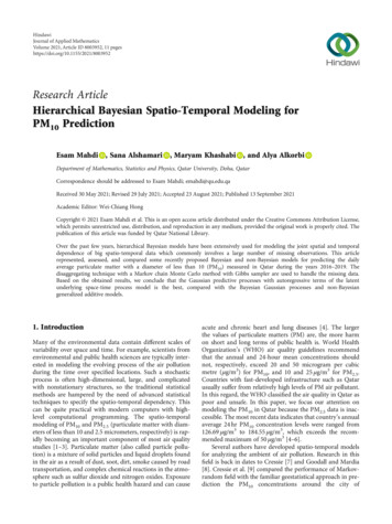
Journal of Applied Mathematics8005Qatar UniversityAl KhorAbu Samra6004002000800Al RuwaisDoha AirportAl WakrahPM106004002000800DukhanMukenis Al KaranaahUmm Said60040020002016 Jul 2017 Apr 2018 Jan 2018 Oct 2019 Jul2016 Jul 2017 Apr 2018 Jan 2018 Oct 2019 Jul2016 Jul 2017 Apr2018 Jan2018 Oct2019 JulTime in hoursFigure 2: Daily PM10 concentrations observed in nine locations over the years 2016-2021.where C ðϕ, κÞ is the n m crosscorrelation matrix betweenηt and η t having elements ½C ij Cðksi s j kÞ, i 1, , nand j 1, , m, and H η ðϕ, κÞ is the m m correlationmatrix of η t so that ½H η ij ½Cðks k s j k ; ϕ, κÞ , for k, j 1, , m. Clearly, the process f ηℓt g shows nonstationarystructure with variance function that is given by′ Varð ηt Þ C ðϕ, κÞH 1η ðϕ, κÞC ðϕ, κÞ:ð11ÞThe advantage of using the nonstationary model in (10)is the flexibility in the ηt surface which is based on m n linear functions of η t . When m is very small compared with n,this will lead to reduce the computational burden, especiallyfor big data which is usually the case of the spatio-temporaldata. Moreover, using nonstationary models usually providesmore accurate results in prediction the nonstationary PM10process. We specify the hierarchical Gaussian predictive processes (GPP) as follows:Zℓt Yℓt εℓt ,Yℓt Xℓt β ηℓt ,ð12Þwhere ηℓt is given in (10). The process fη ℓt g, at the S m knots,can be modeled according to the autoregressive modelη ℓt ρη ℓt 1 ηℓt ,ð13Þwhere η ℓt N m ð0, Ση Þ for ℓ 1, , r, t 1, , T ℓ and Ση σ2η H η . We assume that the initial conditions η ℓ0 has normal distribution with mean zero and covariance matrix Σ0 σ2ℓ H 0 , and both Ση , Σ0 can be obtained from the Matérncovariance function defined in (4), where Ση is an m mmatrix much lower dimensional than Ση of dimension n n.In this case, logarithm of the joint posterior distribution ofthe missing data and the parameters in this case is given by:log pðθ, Y, z zÞTN1 r ℓlog σ2ε 2 ðZℓt Yℓt Þ ′ ðZℓt Yℓt Þ22σε ℓ 1 t 1 N mNlog σ2η log H η 22 rm rð14Þ log σ2ℓ log ðjH 0 jÞ2 ℓ 12 T 1 r ℓ ðη ρη ℓt 1 Þ ′ H 1η ðηℓt ρηℓt 1 Þ2σ2η ℓ 1 t 1 ℓt 1 r 1 ′ 1 η H η log pðθÞ,2 ℓ 1 σ2ℓ ℓ0 0 ℓ0where pðθÞ is the prior distribution for the parameter θ ðβ, ρ, σ2ε , σ2η , ϕ, κ, σ2ℓ Þ and the Gibbs sampling procedureof these parameters can be obtained from the full conditional distributions required provided in the Appendix.
6Journal of Applied MathematicsPM1060040020002016201720182019Daily average of PM10 pollutant by yearPM106004002000Qatar UniversityAbu SamraAl KhorAl RuwaisAl WakrahDoha AirportDukhan Mukenis Al Karanaah Umm SaidDaily average of PM10 pollutant by siteFigure 3: Boxplots of daily average of PM10 concentrations over the years 2016-2019 and by 9 locations in Qatar showing the quartiles; thewhiskers show the farthest observation from the median.3. Numerical Example3.1. Data Description. The data used in this article isobtained from three different sources. The first one was collected by the air pointer and the meteorological station andis managed by the Environmental Science Center at QatarUniversity over the years 2016-2019. It has hourly pollutantincluding PM10 measured in μg/m3, temperature, Temp,measured in degree Celsius, and relative humidity, RH, withseveral missing values.First, we sort the data into an ascending order by date,and then, we impute the missing values of the PM10 by averaging the two nonmissing values before and after this missing value. When two or more successive missing values exist,we impute them by the corresponding monthly average. Wedo the same for the hourly missing values of temperatureand relative humidity. After that, we aggregate the hourlydata into daily data for which we fit our models. Theamended data from this resource is irregular time serieswhich started on the fourth of January 2016 and ended onthe twenty-eighth of August 2019. Table 1 provides a summary statistics of this data. Results suggest that the PM10levels increased during the time, and the majority of missingobservations (with more than 52%) have been occurred during the year 2018.The second source of the data was the regular monthlyobservations obtained from nine meteorological stations overthe years 2016-2019. The total number of observations is 432where the stations are located in the following sites: Qatar University, Abu Samra, Al Khor, Al Ruwais, Al Wakrah, DohaAirport, Dukhan, Mukenis-Al Karanaah, and Umm Said.Figure 1 shows the map locations of 9 meteorological sites.Although this data provides the monthly average values oftemperature in degree Celsius and relative humidity (RH), itdoes not include measures for any type of pollutant. Table 2summarizes the descriptive statistics of this data. We use thisdata to interpolate the daily temperature and relative humidityby disaggregating technique at each location. We also use ourown portable devices to collect daily PM10 values, as a thirdsource of data, over the period of time from November 5thto December 31th of 2020 close to these sites. We use thesedevices to collect and simulate more daily PM10 concentrations over the aforementioned locations. In particular, werecorded the average of the PM10 taken randomly in themorning and evening of each day over this period. Then, weuse this collected data to simulate a new data in each location.
Journal of Applied Mathematics7Table 3: Posterior estimates and 95% credible interval for the parameters of the AR, GP, and GPP models fitted for PM10 concentrationlevels. SD stands for standard 35211.35190.0206(1.3115, 2(-0.0007, 0.0009)(-0.0004, 0.0003)0.01600.01450.0267(-0.0328, 0.0734)σ2ε0.02090.02080.0007(0.0199, 0.0226)σ2η0.01240.01230.0009(0.0107, 0.0144)ϕ0.01680.01680.0000(0.0168, 0.0168)β012.130312.43781.1060(9.7744, 0041(-0.0590, 0.0538)(-0.0209, -0.0062)σ2ε0.00520.00520.0001(0.0050, 0.0054)σ2η15.226212.83937.9727(6.6616, 35.1414)ϕ0.00320.00270.0018(0.0011, 0.0069)β00.47920.47840.0692(0.3425, .0003(-0.0053, -0.0003)(-0.0018, -0.0007)0.97040.97040.0025(0.9654, 0.9754)σ2ε0.00520.00520.0001(0.0050, 0.0054)σ2η1.74501.74530.0256(1.6955, 1.7954)ϕ0.00100.00100.0000(0.0010, 0.0010)Table 4: Validation statistics for the GP, AR, and GAM 95% credible intervalMSE991.04360.15332.82202.04MAE MAPE rBIAS rMSEP79.95 122.4336.37 46.5336.61 48.37916.61 lly, we merge the simulated data with the previous oneand obtained the data that we use in this article.The final data has 1037 observations (see Figure 2)which has three variables (PM10, temperature, and relativehumidity) measured over irregular time over the years2016-2020 in nine spatial locations.The top panel in Figure 3 shows the distribution of thedaily average PM10 concentrations over the years 20162020, whereas the bottom one in the same figure shows theseaverages by the nine sites. Clearly that the distribution of thePM10 concentrations, in all locations, are right skewed withvery high extreme values. Thus, to stabilize the varianceand reduce the departure from normality, we transformthe original scale to square root scale.3.2. Parameter Estimates, Model Validations, Prediction, andComparison Results. The main objective of this research is todevelop a hierarchical Bayesian model that can be used toselect and validate the best model which fits the daily averageof the PM10 air pollutant levels over different locations inQatar. We consider the two covariates, temperature and relative humidity, for spatial interpolation of the PM10 concentration at a new location and any time.First, we use the MCMC algorithm with Gibbs sampler,based on 5,000 iterations discarding the first 1,000 values,to impute the missing data z as explained in Appendix,and then, we utilize this data to predict the values of Zðs ′ ,tÞ at new location s ′ fs1 , ,sn g. The posterior predictivedistribution is ð p z s ′ , t z p z s ′ , t S m , η , θ, z ð15ÞpðS m , η , θ zÞdS m dη dθ,where θ ðρ, σ2ε , σ2η , ϕÞ ′ are the model parameters and η ðη 1 , ,η n Þ ′ (see [17]). We fit the Bayesian GP, AR, andGPP models described in Section 2 using the spTimer package [21, 23] and compare these models with the nonBayesian generalized additive model (GAM) using the Rpackage mgcv [24–26]. We use the crossvalidation methodto evaluate the predictive performance of these models.Here, data at locations ðs1 , ,sm Þ where m n are used tofit the model while data at other sites ðsm 1 , ,sn Þ are used
8Journal of Applied Mathematics600PM1040020002016 Jul2017 Apr2018 JanTime in hours2018 Oct2019 JulFigure 4: Time series plots of the true (blue) and fitted values (green) at one randomly chosen location (Qatar 1.051.2Longitude4.551.451.6(b)Figure 5: Spatially interpolated plots of the daily average of PM10 concentration levels (a) and their standard deviations (b) obtained fromthe AR model for the 29th of March 2018 (top graphs) and 15 May of 2019 (bottom graphs). Actual values and associated locations aresuperimposed in plots, respectively.
Journal of Applied Mathematics9to assess the model using the mean squared error (MSE),mean absolute error (MAE), mean absolute prediction error(MAPE), relative bias (rBIAS), and relative mean separation(rMSEP) defined, respectively, as follows:MSE 1 N ðz ̂z Þ2 ,N i 1 i i4. ConclusionN1 jz ̂z j,N i 1 i i 1 N ðz i ̂z i Þ ,MAPE N i 1zi MAE rBIAS 1 N ðzi ̂z i Þ , zN i 1rMSEP 1 N ðz i ̂z i Þ2 , N i 1 ̂z z itrend surfaces of the PM10 values with their standard values,we illustrate a prediction map for the 29th of March 2018 and15 May of 2019 over a one-kilometer square grid (seeFigure 5). Obviously, the graphs show that the GPP modelcorrectly represented the PM10 concentration level over thespace and time.ð16Þwhere N is the total number of nonmissing observations, ̂z iis the posterior predictive value of z i , and z , ̂z z i are thearithmetic means of z i , ̂z i for i 1, , N.Specifically, we use the data from Abu-Samra and Dohaairport stations with 2 1037 2074 observations for validation purposes. The data from the remaining six stations with7 1037 7259 total number of observations are used formodel fitting (see Figure 1). The parameter estimates (posterior) for the Bayesian spatio-temporal models are given inTable 3. The 95% credible intervals for the parameters suggest that most of regression parameters for the AR and GPmodels are statistically significant, whereas the GPP modelsuggest that the variables are significant. In all models, thenugget effect σ2ε is small. On the other hand, the spatialdecay parameter ϕ 0:0033 for GP model and ϕ 0:001for GPP model suggesting that the effective ranges willapproximately be 909 and 3000 kilometers, respectively.These two values are unusual associated with very large spatial variance values (σ2η ) suggesting that the PM10 concentrations in Qatar are not significantly different over the space.After fitting the three models, we perform the crossvalidation and select the best one. Table 4 summarized the validation statistics for the GAM, GP, and AR models. Clearly,the MSE, MAE, MAPE, rBIAS, and rMSEP are smaller forthe Bayesian spatio-temporal methods providing better predictive performance compared to the non-Bayesian additivemodel. For example, the Bayesian AP, GP, and GPP modelsreduced the MSE by about 63.7%, 66.4%, and 79.6%, respectively, compared with the non-Bayesian GAM model. Weconclude from this table that the Bayesian spatio-temporalGPP model is the best model that can be used to predictthe PM10 concentr
and Mardia [13] used short-term spatio-temporal predictive analysis for modeling the PM 2.5 and PM 10 concentration levels. Zidek et al. [3] presented predictive distributions on nonmonitored PM 10 values in Vancouver, Canada. Smith et al. [14] proposed a spatio-temporal model to predict the weekly averages of particulate matter concentrations .