Transcription
Mathematical Models for Stock PinningNear Option Expiration DatesMarco Avellaneda , Gennady Kasyan†andMichael D. Lipkin‡June 24, 20111IntroductionThis paper discusses mathematical models in Finance related to feedback between options trading and the dynamics of stock prices. Specifically, we considerthe phenomenon of “pinning” of stock prices at option strikes around expirationdates. Pinning at the strike refers to the likelihood that the price of a stockcoincides with the strike price of an option written on it immediately before theexpiration date of the latter. (See Figure 1 for a diagrammatic description ofpinning).Conclusive evidence of stock pinning near option expiration dates was givenby Ni, Pearson and Poteshman (2005) [8] based on empirical studies. Theoretical work was done by Krishnan and Nelken (2001) [5], who proposed amodel to explain pinning based on the Brownian bridge. Later, Avellaneda and CourantInstitute and Finance Concepts LLCInstitute‡ Columbia University and Katama Trading LLC† Courant1
15.00Trajectory B pinnedShare PriceB.Trajectory A did not 12.50A.Option expirationFriday, (3rd Friday ofthe month).Time 10.00Figure 1: Stock price pinning around option expiration dates refers to the trajectory B which finishes exactly at an option strike price on an expiration date.2
Lipkin (2003)[1] (henceforth AL) formulated a model based on the behavior ofoption market-makers which impact the underlying stock price by hedging theirpositions. AL consider a linear price-impact model namely, S E·QSwhere S is the price, E is a constant (elasticity of demand), and Q is the quantityof stocks demanded. According to AL, pinning is a consequence of the demandfor Deltas by market-makers in the case when the open interest on a particularstrike/expiration is unusually high. In this paper, we consider more generalnon-linear impact functions which follow power-laws, i.e., we shall assume that S E · QpS(1)where p is a positive number. Such impact models have been investigated bymany authors in Econophysics; see, among others, Lillo et al.[6], Gabaix[2]and Potters and Bouchaud [9].1 In the particular context of pinning aroundoption expiration dates, Jeannin et al. [4] suggested that the results of ALwould be qualitatively different in the presence of non-linear price elasticity and,specifically, that pinning would be mitigated or would even disappear altogetherfor sufficiently low values of p.The goal of this paper is twofold: first, we review the issue of pinning aroundoption expiration dates, both from the point of view of the AL model andfrom empirical data, and, second, we analyze rigorously the non-linear model(2), expanding on the work of AL along the lines of Jeannin et. al. We find,in particular, that there exists a “phase transition” of sorts – in the sense ofStatistical Physics – associated with the model’s behavior in a neighborhood of1 Toour knowledge, there is not yet a clear consensus for the correct value of the exponentp, as price impact is difficult to measure in practice.3
p 1/2. In fact, for p 1/2, there is no stock pinning around option expirationdates.The case p 1/2 is first analyzed numerically by Monte Carlo simulation.We show that the probability of pinning at a strike based on model (1) satisfiesPpinning c1 e c2(p 1/2) (1 o(1)) ,(2)where Ppinning is the probability that the stock price coincides with a strike levelat expiration, for some constants c1 , c2 . This suggests that that the behavior ofthe pinning probability is C around p 1/2, but not analytic. In other words,there is an infinite-order phase-transition in the vicinity of p 1/2, accordingto the value of the exponent in (1). For p 1/2 price trajectories behave like“free” random walks; for p 1/2, there is a non-zero probability that theyconverge to an option strike level.The outline of the paper is as follows: first, we review empirical results onthe existence of pinning. Then, we discuss the AL case, p 1, for which wehave a complete analytical solution. Then, we consider general exponents p.We present numerical evidence of equation (2) and give a rigorous justificationof (2) for all values of the exponent p, 0 p 1 in the form of a theorem.The mathematical techniques used in the proof consist of Large Deviationestimates for small-noise perturbation of dynamical systems (a.k.a. VentselFreidlin theory) and a rigorous version of the real-space Renormalization Group(RG) technique, which is the key element in deriving (3) and, in particular, thebehavior of the pinning probability around the critical point p 1/2.4
2Empirical evidence of pinningIn a comprehensive empirical study on the behavior of prices around optionexpirations, Ni, Pearson and Poteshman (2003) (henceforth NPP)[8] consideredtwo datasets: IVY Optionmetrics, which contains daily closing prices and volumes forstocks and equity options traded in U.S. exchanges from January 1996 toSeptember 2002 Data from the Chicago Board of Options Exchange (CBOE) from January1996 to December 1001 providing a breakdown of option positions amongdifferent categories of traders for each product. This dataset divides theoption traders into 4 categories: market-makers, firm proprietary traders,large firm clients and discount firm clients. After each option expiration,the data reveals the aggregate positions (long, short, quantity) for eachtrader category.NPP separated stocks into optionable stocks (stocks on which options hadbeen written on the date of interest) and non-optionable stocks. The data analyzed by NPP consists of at least 80 expiration dates. There were 4,395 optionable stocks on at least one date and 184,449 optionable stocks/expirationpairs. There were 12,001 non-optionable stocks on at least one date and 417,007non-optionable stock/expiration pairs.The NPP experiments consisted in studying the frequency of observations ofclosing stock prices which coincide with strike prices or with multiples of 2.5,or 5 (which are the standardized strike levels for U.S. equity options) on eachday of the month. By separating stocks into optionable and non-optionable andlooking at the frequency with which the price closed near such discrete levels,NPP established statistically that stocks are more likely to close near a strike5
level on option expiration dates than on other days. They also showed that pinning is definitely associated with optionable stocks (see Figures 2 and 3). NPPalso compared the cases of non-optionable stocks which later became optionable and optionable stocks that were previously non-optionable, The empiricalevidence being that the former category is not associated with pinning and thelatter is (Figures 4 and 5).Percentage of non-optionable stocks closing within 0.25 ofan integer multiple of 513%Expiration Friday1 2.5121 1.511-1 0-9-8-7-6-5-4-3-2-10r e la t i v e t r a d i n g d a t e f r o m1234567891 0o p t io n e x p ir a ti o n d a t eRelative Trading Date from Option Expiration Date(Courtesy: Ni, Pearson & Poteshman)Figure 2: The different bins correspond to frequencies of instances for which theclosing price of a non-optionable stocks is within 0.25 of a multiple of 5. Eachtrading day of the month is labeled with an integer between -10 and 10, andexpiration Friday corresponds to the label 0. Notice that there is no appreciabledifference between the frequencies associated with different days of the month,suggesting that closing near a level which is a multiple of 5 dollars is equallyprobable for different days of the month for non-optionable stocks.6
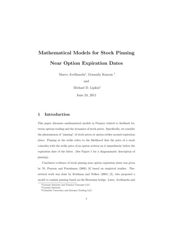
Percentage of optionable stocks closing within 0.25 ofa strike price%191 8.5181 7.5-1 0-9-8-7-6-5-4-3-2-10r e la t i v e t r a d i n g d a t e f r o m1234567891 0o p t io n e x p ir a ti o n d a t eRelative Trading Date from Option Expiration Date(Courtesy: Ni, Pearson & Poteshman)Figure 3: Frequencies of observations of prices of optionable stocks closing within 0.125 of a strike price. The data shows that the likelihood that a price endsnear an option strike price is significantly greater on expiration Friday, comparedto other days.7
Non-optionable stocks that later became optionable closingwithin 0.125 of an integer multiple of 2.501 2.5121 1.5%111 0.510-1 0-9-8-7-6-5-4-3-2-10r e la t i v e t r a d i n g d a t e f r o m12345678o p t io n e x p ir a ti o n d a t eRelative Trading Date from Option Expiration DateFigure 4: Same as in Figure 2 for non-optionable stocks which later becameoptionable. There is no evidence of pinning.891 0
Optionable stocks that were previously non-optionableclosing within 0.125 of an integer multiple of 678relative trading date from option expiration dateFigure 5: Same as in Figure 3 for optionable stocks which were previously nonoptionable. Notice the peak at bin 0 which is associated with pinning.9910
The conclusions of NPP are that, based on frequencies of observations, optionables are more likely to end near a strike level (which is a multiple of 2.5)on expiration dates, whereas non-optionables have the same likelihood of closingnear a multiple of 2.5, regardless of whether the day corresponds to the thirdFriday of the month or not.3A model based on market microstructureConsider the case of the stock of J.D. Edwards (JDEC) during February andMarch 2001. This stock experienced an unusual volume in options with Marchexpiration during the last days of February as shown in Figure 6. Following atrade of 4,000 contracts on February 17, a very large volume of March optionswith strike price 10 were traded on February 27, bringing the total open interest for puts and calls on the 10 line to 56,000 contracts. Recalling that theequity option contracts correspond to 100 shares, the total notional shares corresponding to the options is 5.6 million shares. On the other hand, the averagetraded volume in stocks was approximately 1 million shares.The existence of this large open interest in the 10-strike options is important,since the large increase in open interest will potentially increase the tradingvolume. Figure 7 shows the chart of the stock during the same period of time.We notice from Figure 7 that, after the large option trade on February 27, thestock price became less volatile and converged to the price of 10 which is thestrike price of the options with large open interest.To connect the stock price dynamics to the increase in open interest inoptions, we posit that there is a “feedback effect” due to the demand for Deltasfor hedging the options. To be more precise, we make the following assumptions.10
2/9/2/ 20011 1/22/ 0 013 1/22/ 0 015 1/22/ 0 017 1/2/ 20 019 1/22/ 0 021 1/22/ 0 023 1/2/ 20 025 1/22/ 0 027 1/203/ 011/203/ 0 13/23/ 00 15/203/ 0 17/203/ 0 19/3/ 20011 1/3/ 20 013 1/23/ 0 015 1/2001ContractsJDEC 2001 Mar 10Put & Call Open Interest6000050000400003000020000100000DateFigure 6: Evolution of the open interest in March options on JDEC with strike 10, with a very volume transacted on February 27.11
JDEC in March 20011211.51110.5109.502/1602 /01/2002 /01/2102 /01/2202 /01/2302 /01/2602 /01/2702 /01/281/ /013/22/ 0013/25/ 0013/26/ 0013/27/ 0013/28/ 0013/29/ 0013/12 200/3 1/203 001/1303 /01/1403 /01/1503 /01/16/019Large trade in Mar 10options on this dayFigure 7: Evolution of the price of JDEC during the same period. We observethat the volatility of the stock diminishes after February 27 and the stock priceconverges to 10 as the March expiration approaches.12
After the increase in open interest1. The open interest becomes unusually large relative to normal volumes2. A significant fraction of market-makers is long options (i.e. they boughtthe block of options that traded).The two assumptions have the following consequences: first, since the openinterest on the particular strike/maturity is large, the notional number of underlying Deltas (in the sense of Black-Scholes) is large compared with typicaltrading volumes. In particular, hedging the options – if one were to hedge –would imply trading relatively large quantities of stocks in relation to normaltrading volume.Second, the fact that market-makers are long options means that they arelong Gamma. Delta-hedging implies that they will sell the stock when the pricerises and buy the stock if the price drops. Delta-hedging in large amounts mayaffect the underlying stock price and drive it to the strike level.What happens if we assume that assumption 1 holds but not assumption2? If market-makers are only marginally long, then the demand for stock inthe pattern described above may not be present and there is not price pressurepushing the stock to the strike price. Also if market-makers are predominantlyshort options, they may choose not to hedge or to hedge only partially. This isdue to the fact that delta-hedging a short-gamma position implies buying highand selling low. On the other hand, if market-makers are long options they earnmoney by hedging frequently and thus may indeed impact the stock price. Thisis the essence of the AL model.In order to formulate a quantitative model, we consider the following priceimpact relation:13
D S E·S V pD1, V sign(D)(3)where S is the stock price, D is the demand, V is the average daily tradingvolume and p is an exponent. The choice of the parameter p is a fundamentalquestion in Econophysics, with different authors proposing different values: p 0.22 in [6], p 1/2 in [2], and p 1.5 in [9].4AL modelWe assume that p 1 and thatD OI δ(S, t)dt t(4)where OI represents the open interest on the strike of interest δ is the BlackScholes delta, or hedge-ratio for an option in terms of number of shares of theunderlying asset. According to the Black-Scholes formula,Zd1δ N (d1 ) 2e x2dx ,2πd1 1 σ τ Seµτσ2 τln() K2 ,where σ is the implied volatility, µ is the carry rate, S is the stock price, K is thestrike price and τ T t is the time left before the option expires. For simplicity,we focus the analysis on the strike price with largest open interest and consideronly one potential pinning point.2 From the above considerations, it can beshown that the stochastic differential equation describing the phenomenon ofstock pinning to leading order is [1],2 In practice, the analysis might involve more than one strike price if the open interest islarge in several contracts.14
dy t))2E · OI y a(T t) (y a(Tpe 2σ2 (T t) dt σdW, V 2πσ 2 (T t)3where y ln(S/K) and a µ σ22 .(5)Since we expect the system to be drivenby the drift’s singularity, we assume that a 0 and introduce the dimensionlessvariablesy ,σ T S0y1 0 lnz0 Kσ Tσ TE · OI β V 2πσ 2 Ts t/T.z (6)With these new variables the SDE in (6) becomesdz 4.1z2βz 2(1 s)eds dW.(1 s)3/2(7)Solution of the modelWe set τ 1 s and seek positive solutions of the Fokker-Planck equation F1 2Fβz z2 F e 2τ, τ2 z 2 zτ 3/2(8) 1zF (z, τ ) exp φ .ττ(9)of the formSubstituting this form in equation (9), we find that φ φ(ζ) satisfies the SDEφ ζφ0 φ00(φ0 )2 2βζe τ22τ 3/215ζ22φ0 0.(10)
Since, as τ 0 the second term in the equation is formally the dominant one,we consider the eikonal equation(φ0 )2 2βζe ζ22φ0 0,which has the explicit solutionφ(ζ) 2βe ζ22.As it turns out, this function also makes the O(τ 3/2 ) term vanish. Thereforez2F (z, τ ) e2β e 2ττ.(11)is an exact solution of equation (8). In particular, the functionz2G1 (z, τ ) 1 F (z, τ ) 1 e2β 2τ eτ(12)satisfies the Fokker-Planck equation (8), with initial conditionlim G1 (z, τ )τ 0 0 z 6 0 1 z 0.(13)Hence, the analytical formula for the pinning probability isz2no 0Ppinning Prob. lim z(s) 0 z(0) z0 1 e 2β e 2 .s 1(14)We note that this formula contains two adjustable parameters: z0 , the logdistance from the current price to the option’s strike price measured in standarddeviations, and β, the coupling constant, which is proportional to the dimensionless open interest (OI/ V ) and inversely proportional to the stock16
volatility and the time-to-expiration. In particular, it suggests that the presence of a large open interest gives rise to a large probability of pinning, as shownin Figure 8.Pinning Probability0.90.80.7prob0.60.5Zo 0.5Zo 00.40.30.20.100.05 0.1 0.15 0.2 0.25 0.3 0.35 0.4 0.45 0.5 0.55 0.6 0.65 0.7 0.75BetaFigure 8: Pinning probability for the AL model (equation (14)) as a function of the dimensionless parameter β V E·OI. The curves show the function2πσ 2 Tfor z0 0 and if z0 0.5.5Empirical evidence in favor of the AL modelWe know from NPP that pinning is associated with option expirations; and thisis consistent with our model. However, we made a strong additional assumption17
to justify pinning: namely that market-makers are net long options near theexpiration date. But is this actually the case?We asked Ni, Pearson and Poteshman to analyze pinning along the linesof their empirical study taking into account the positions of market-makers,which is feasible to do using CBOE data. Their results, show in Figures 9 and10, confirm our second hypothesis: if market-makers are net long options, thefrequency of pinning at option expiration dates is much higher than if marketmakers are net short.Observations with market-makers net long( 0.125)Figure 9: Frequency of pinning at the strike for expirations in which marketmakers are net long options. (Courtesy of Ni, Pearson and Poteshman (2003)).Additional empirical validation of the model was done by Lipkin and Stan18
Market-makers net shortFigure 10: Frequency of pinning at the strike for expirations in which marketmakers are net short options. (Courtesy of Ni, Pearson and Poteshman (2003)).19
ton (2006) [7] in unpublished work. Using the IVY OptionMetrics data, theyobtained clear empirical evidence of monotonicity of the pinning probability asa function of OI/( V σ), consistently with Figure 8 and equation (14); seeFigure 11.6Power-law modelWe turn to the case in which price/demand elasticity is non-linear and follows apower law. Based on the previous considerations, we propose the generalizationof the AL model:dS E OIS 1 δ(S, t) V t p sign δ(S, t) t dt σdW(15)or, in dimensionless variables,dz pz 2β z p sign(z) 2(1 s)eds dW,3p/2(1 s)the coupling constant being β (16)E OI. V p (2πσ 2 T )p/2In (16), the drift of the SDE corresponds to a “restoring force” that blows upas s 1, favoring pinning at z 0 for s 1. However, this force is localized ina small neighborhood of the origin, due to the presence of the Gaussian cutoffpz 2function e 2(1 s) . The behavior of Z(s) as s approaches 1 is the result of atradeoff between these two effects: the restoring force which favors pinning andthe localization with diffusion, which favors not pinning.To formulate a hypothesis about the model’s behavior, we performed MonteCarlo simulations to calculate numerically the probability of pinning for a trajectory starting at z0 0 for different values of p and for fixed β 0.2. Theresults indicate that there is no pinning for p 0.5 and that pinning occurs forp 0.5 following equation (3). The functional form (2) is strikingly apparent20
0.080.090.100.110.120.130.14Pinning Probability (By Quartile)00.000310.00120.00346Open Interest / (Average Daily Volume Implied Volatility)Figure 11: Empirical result showing the monotonicity of the pinning probabilityversus β VOI σ . (Courtesy of Lipkin and Stanton (2006) [7].211
from the simulations, as seen in Figures 12, 13 and 14.Figure 12: Pinning probability as a function of the parameter p for the powerlaw impact model. Each point corresponds to a simulation with a different valueof p, with more points used near p 0.5.The associated Fokker-Planck equation for general values of p is given by F1 2Fβ z p sign(z) pz2 F e 2τ.2 τ2 z zτ 3p/2(17)A simple analytic solution of this equation such as (14) does not appear to existfor p 6 1. Nevertheless, suppose that (17) admits a solution with the boundarycondition (13), which we denote by Gp (z, τ, β). Dimensional analysis impliesthat Gp (z, , β) satisfies the RG identity22
Figure 13: Same as Figure 12, but with pinning probability plotted on a logscale.23
Figure 14: Same as Figure 12. Logarithm of the pinning probability plotted1against 2p 1.24
Gp αz, α2 τ, β Gp z, τ,β α2p 1.(18)Inspired by the numerical results, we shall use Large Deviations and RGanalysis to study the model rigorously for 1/2 p 1.We shall prove the following result:Theorem: Let z(s) be the solution of the stochastic differential equationdz pz 2β z p sign(z) 2(1 s)eds dW, z(0) z0 , 0 s 1(1 s)3p/2(19)with β 0.(i) If p 1/2, there is no pinning, i.e.,noP rob lim z(s) 0 z(0) z0 0s 1for all z0 .(ii) (Lower bound). Let 0.5 p. There exists positive constants C1 and C2 ,depending only on β, such thatnoC2P rob. lim z(s) 0 z(0) 0 C1 e (p 0.5) .s 1(20)(iii) (Upper bound). Let 1/2 p 1. There exist constants C3 , C4 dependingonly on β but not on p such thatnoC4P rob. lim z(s) 0 z(0) 0 C3 e (p 0.5) .s 1In particular, there is no pinning for p 1/2.25(21)
6.1Absence of pinning for p 1/2.The magnitude of the drift V (z, s) of the SDE (19), satisfiesβ z p pz2βe p/2β2τe p.τpττ 3p/2If p 1/2, V (z, s) is square-integrable in the interval [0, 1] and, furthermore,Z12(V (zs , s)) ds β02Z1β2ds .(1 s)2p1 2p(22)0Therefore, for any constant c 1, we haveE eR1c (V (zs ,s))2 ds 0 β2 ec 1 2p , so the drift satisfies Novikov’s condition [3] for absolute continuity of the processz(·) with respect to standard Brownian motion. This rules out pinning forp 0.5.6.2Technical lemma for the lower boundOur proof of Part (ii) of the Theorem makes use of a technical lemma whichprovides an upper bound for the exit probability of the process z(s) from a“standardized” parabolic space-time region.Lemma 1: Let Ω denote the region in the z, s-plane defined by(i) 0 s 3/4, (ii) z 2 1 s,(see Figure 15) and let θ be the first exit time of z(·) from Ω. Thenlim supβ 1ln P rob. {θ 3/4 or z(3/4) 1/2 z(0) 1} Iβ26(23)
12ZtFigure 15: The parabolic region Ω used in the proof of Lemma 1. The mainstatement of the lemma is that, for large values of β, paths which start at z 1are most likely to end at z(3/4) 1/2 without exiting Ω. In particular, pathswhich either (1) exit before time t 3/4, or (2) end outside z(3/4) 1/2have exponentially small probability of the order of exp( βA), where A is theVentsel-Freidlin action. This action is uniformly bounded away from zero.27
where I is a constant independent of p and β.Proof: We setξ(t) z(t/β), 0 t 3β/4.This process satisfies the stochastic differential equationdξ(t) U (ξ(t), t)dt dW (t/β)1 U (ξ(t), t)dt dZ(t),β where U (ξ, t) 0 t 3β/4.(24)ξ2 ξ p sign(ξ)e 2(1 t/β)(1 t/β)3p/2and Z(t) is a Wiener process. If we consideronpthe region Ωβ (ξ, t) : ξ 2 1 t/β, 0 t 3β4 , the estimate that we seekcorresponds to the first-exit time of (ξ(t), t) from this region, where ξ(t) is adiffusion process with small diffusion constant 1 .βAccording to Ventsel-Freidlin (1970) [10], the probability that a trajectoryξ(·) remains in a tube-like neighborhood of a given path γ(t), 0 t untiltime t 3β4is given, for β 1, by the “action asymptotics”P {tube around γ(·)} e βA(γ)with1A(γ) 2Z 2(γ 0 (t) U (γ(t), t)) dt.0We claim that the actions corresponding to the event of interest are boundeduniformly bounded away from zero. To see this, we note that U is uniformlybounded in the region of interest and satisfiesU (ξ) ξ p e 2 .28
In particular, the characteristic paths ξ 0 U (ξ, t) are such that ξ(t) ω(t) where ω 0 ω p e 2 . The latter ODE has the explicit solutionω(t) (1 p)11 p 1 1 p(ω(0))1 p 2 e t.1 pNotice that as t , the latter trajectory hits ω 0 in finite time t (25)3β4 .Therefore, the characteristic (“zero-diffusion”) paths starting in the interval ξ(0) 1 also reach zero in finite time.3 For β sufficiently large, they exit theregion through ξ 0 at time t 3β4 .This shows that the action A(γ) of pathswhich exits Ωβ before t 3β/4, or with an absolute value greater than 1/2 fort 3β/4, is bounded from below by a positive constant, I. We leave it to thereader to verify that the constant can be chosen independently of p and β, thusestablishing the Lemma.6.3Proof of the lower boundWe consider the parabolic region Γ (z, s) : z 2 1 s, 0 s 1 ,(26)which is shown in Figure 16. The proof of the lower bound is based on estimatingthe probability that the path z(·) remains inside the region Γ, which clearlyimplies pinning.Let D be the event that the space-time process (z(s), s) remains inside Γ,i.e.,D {(z(·), ·) Γ } ,and let tn 1 (1/4)n , n 0, 1, 2. We denote the probability measure asso3Asimilar comparison argument can be made for p 1.29
ZtFigure 16: Representation of the region Γ used in the proof of the lowerbound. The strategy of the proof is to estimate the probability that a pathx(s), 0 s 1 remains confined to the region and also passes through thehighlighted segments. The region can be viewed as an infinite union of parabolically “homothetic” regions which map to the standardized region Ω after thescaling transformation (28).30
ciated with z(·) by Pβ to emphasize the dependence on the coupling constant.Then Pβ (D) PβD; z(tn ) Z1/2 Pβ {(z(s), s) Ω; z(t1 ) x} Pβ 1, n,2nD; z(tn ) 1, n 1 z(t) xdx12n 1/2 1 ce βI Pβ z(s) 2 1 s, s 3/4, z(3/4) 1/2 1 ce βI Pβ1 (D),(27)where β1 β22p 1 . The third line follows from Lemma 1, where c is a constantindependent of β. The last line follows from the fact that the diffusion equationgoverning the process is invariant under the scaling transformationz1 2zτ1 4τβ1 β22p 1 ,(28)(see equation (18)) . Iterating this last result, we obtain the lower boundPβ (D) Y2p 1 n)1 ce Iβ(2.n 031(29)
Let us evaluate this infinite product as a function of p. We have4ln Pβ (D) X 2p 1 n)ln 1 ce Iβ(2n 0 c Xn 0Z ce Iβ(22p 1 )ne Iβ(22p 1 )x c2 X 2Iβ(22p 1 )ne 2 n 0c2dx 22p 1 xe 2Iβ(2)dx (c c2)200 Z 11 c(2p 1) ln 2Z e Iβudu c2u1Z c2e 2Iβu du (c ).u21(30)This establishes the desired lower bound for the pinning probability for p 1/2.Notice that this implies that there is a “phase transition” at p 1/2, since thelower bound implies that pinning occurs for p greater than 1/2.It remains to show that the exponential form associated with the lower boundalso holds as an upper bound, as suggested by the numerical experiments.6.4Two more technical lemmasWe begin with:Lemma 2: Let U1 (z, τ ) and U2 (z, τ ) be two positive functions such that U1 (z, τ ) U2 (z, τ ) for all (z, τ ), and let ψ0 (z) be an even function which is decreasing forz 0. Let ψi , i 1, 2 denote the corresponding solutions of the Cauchy problem ψi1 2 ψi ψi sign(z)U1, z R τ 0, τ2 z 2 z4 Weuse the estimate Pn 1f (n) Rf (x)dx for non-negative decreasing functions f (x).032
with ψi (z, 0) ψ0 (z), i 1, 2. Then,ψ1 (z, τ ) ψ2 (z, τ ) z τ.Proof: The proof follows immediately from the Maximum Principle applied tothe PDE satisfied by the function ψ1 (z, τ ) ψ2 (z, τ ).Lemma 2 is useful to formalize the intuition that, as p increases, the probability of pinning should increase as well. To show this, we introduce a “modifieddrift” which is always greater than unity (as opposed to the drift in the model,which may take small values).Let Gp (z, τ, β) represent the solution of the Fokker-Planck equation (17)with initial conditionGp (z, τ, β) 1 if z 0 0 if z 6 0,(31)and let Ĝp (z, τ, β) be the solution of the auxiliary PDE Ĝp1 2 Ĝp Ĝp βsign(z)U (z, τ )p, τ2 z 2 zwhereU (z, τ ) 1 z τ32z2e 2τ ,satisfying the same boundary conditions (31). (The modified drift alluded toabove is β sign(z) U (z, τ )p .) Lemma 2 implies thatGp (z, τ, β) Ĝp (z, τ, β).Moreover, since the function 1 U is greater than 1, (1 U )p is an increasing33
function of p. Hence, also by Lemma 2, we haveĜp (z, τ, β) Ĝ1 (z, τ, β).(32)Let E(·) denote the expectation value with respect to the probability distribution of z(s). To evaluate the right-hand side of (32), we use Girsanov’s theoremand the Cauchy-Schwartz inequality:Ĝ1 (z, τ, β) 1 R βsign(z(s))dW β22 τ E e1 τ; lim z(s) 0 z(1 τ ) zs 1 1/2 R1 2h noi1/2βsign(z(s))dW β 2 τ E e 1 τ E lim z(s) 0 z(1 τ ) zs 1 eτ β221/2[G1 (z, τ, β)].Therefore, using equation (14), we haveLemma 3.Ĝp (z, τ, β) e6.5τ β221/2[G1 (z, τ, β)] eτ β22"z22β e 2τ1 exp τ!#1/2(33)Proof of the upper bound1We make use of the renormalization identity (18) with α 2 2p 1 . Accordingly, Gp z 212p 1,τ 222p 1 , β Gp βz, τ,2 ;so 12Gp z 2 2p 1 , τ 2 2p 1 , 2β Gp (z, τ, β) .34(34)
In particular, the probability of pinning starting at z 0 satisfies 2P rob. {z(1) 0 z(0) 0} Gp (0, 1, β) Gp 0, 2 2p 1 , 2β .(35)We now make use of Lemma 3. Accordingly,P rob. {z(1) 0 z(0) 0} 2Gp 0, 2 2p 1 , 2β 2Ĝp 0, 2 2p 1 , 2β"#1/24β eβ 2/2β 2 /2 1 e12 2p 1 2 β e 2 2(2p 1)p β 2 /2 ln 22 βee 2(2p 1) ,1(36)which is what we wanted to show. This concludes the proof of the upper boundfor p 1/2. The absence of pinning at exactly p 1/2 follows from similarconsiderations, since G1/2 (z, τ, β) Ĝp (z, τ, β) for any p 1/2.7ConclusionsThe model for stock pinning near option expiration dates introduced in Avellaneda and Lipkin (2003) was generalized to the case of non-linear, power-law,price impact functions. The price trajectories of stocks are affected by Deltahedging by market-makers which, in the case of large number of options, canimpact the price of the stock, driving it to the strike price.Mathematically, pinning is described by a stochastic differential equ
Mathematical Models for Stock Pinning Near Option Expiration Dates Marco Avellaneda , Gennady Kasyan y and Michael D. Lipkinz June 24, 2011 1 Introduction This paper discusses mathematical models in Finance related to feedback be-tween options trading and the dynamics of stock prices. Speci cally, we consider