Transcription
Image EnhancementPoint OperationsGrey-Scale MappingDigital Image ProcessingLectures 17 & 18M.R. Azimi, ProfessorDepartment of Electrical and Computer EngineeringColorado State UniversityM.R. AzimiDigital Image ProcessingHistogram Modeling
Image EnhancementPoint OperationsGrey-Scale MappingHistogram ModelingArea 2: Image EnhancementGoal:To manipulate an image in order to improve its visual appearance or“quality”and prepare it for high level processing and analysis by anautomated system or a human expert.The process involves devising a sequence of operations for various taskse.g., removing the effects of undesirable noise/interference, edgesharpening, pseudo-coloring, interpolation and magnification,multi-spectral processing, and geometrical operations.The operations are ad-hoc i.e. that they do not consider any priorknowledge about the imaging systems. An acceptable result is typicallyobtained after several trials that may involve fine-tuning the parametersof a particular operation or even trying different algorithms. The criterionfor converging to an acceptable result is based upon the subjectivejudgement of the human observers.M.R. AzimiDigital Image Processing
Image EnhancementPoint OperationsGrey-Scale MappingHistogram ModelingPoint OperationsThe operations used can be categorized into five general categories:Point operationsNeighborhood or Spatial operationsTransform-based operationsMulti-spectral operationsGeometric operations.Point OperationsThese memory-less operations are used for contrast enhancement bymapping the pixel intensities of an image. This is done irrespective of thespatial location of the pixels.There are two general types of point operations namely grey-scalemapping and histogram modeling schemes.M.R. AzimiDigital Image Processing
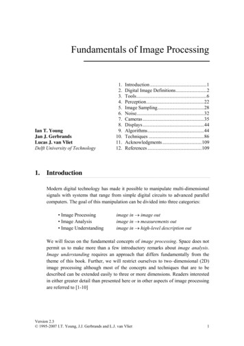
Image EnhancementPoint OperationsGrey-Scale MappingHistogram ModelingGrey-Scale MappingThe grey-scale mapping transforms the original image pixel intensityx {xk , k [0, K 1]} into the transformed image pixel intensityy {yl , l [0, L 1]} usingy f (x)where f (·) is a user-defined (based upon the histogram of the originalimage) grey-scale mapping that can be a linear or nonlinear, one-to-oneor many-to-one function. Since typical digital images have finite numberof grey levels (e.g., K 256), this mapping can easily be implementedusing a look-up table operation.Figures 1(a) and 1(b) show a low contrast image taken under poorlighting condition and its corresponding histogram, respectively. Thelargest intensity in this image is xK 51 which explains why the imageis predominantly dark. To stretch the contrast we use a simple linearmappingy ax,a 1M.R. AzimiDigital Image Processing
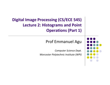
Image EnhancementPoint OperationsGrey-Scale Mapping(a)Histogram Modeling(b)Figure 1The effect of this simple mapping, for a 5 (chosen to make mappingone-to-one), is shown on the histogram in Figure 2(a). Figure 2(b) showsthe resultant image that clearly exhibits better visual appearance thanthat in Figure 1(a). Although histogram is stretched into a wider greylevel range, there are a large number of bins with zero values.M.R. AzimiDigital Image Processing
Image EnhancementPoint OperationsGrey-Scale Mapping(a)Histogram Modeling(b)Figure 2To generalize this idea we use piece-wise linear grey-scale transformationsfor a wide variety of tasks including: contrast stretching, clipping andthresholding, segmentation and digital negative operations.M.R. AzimiDigital Image Processing
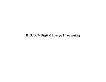
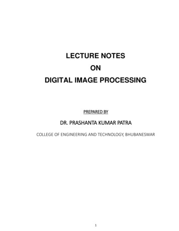
Image EnhancementPoint OperationsGrey-Scale MappingHistogram ModelingA typical piece-wise linear mapping with three segments with slopes a, band c is ax0 x xk1 b(x xk1 ) l1 xk1 x xk2y c(x xk2 ) l2 xk2 x xKwhere xK is the maximum intensity in the original image. The number ofline segments is decided based upon the shape and number of “modes”of the histogram. For instance, Figure (1) represents has a unimodalhistogram while the GOES 8 visible satellite image in Figure 3(a) has abimodal histogram (see Figure 3(b)) corresponding to two separateintensity regions. The values xk1 and xk2 are typically placed at thevalleys of the histogram or boundaries of the modes.M.R. AzimiDigital Image Processing
Image EnhancementPoint OperationsGrey-Scale Mapping(a)Histogram Modeling(b)Figure 3Line segments with slopes greater than one result in contrast stretchingin the corresponding region while slope values less than one lead tocompression of the intensity region (see Figure 4(a)). The resultantimage is shown in Figure 4(b) which exhibits a better definition of cloudshadow areas and low intensity features.M.R. AzimiDigital Image Processing
Image EnhancementPoint OperationsGrey-Scale Mapping(a)Histogram Modeling(b)Figure 4Effect on HistogramThe relationship between the histograms of original image, hX (x), andmapped image, hY (y), as a function of transformation, f (·), can bedetermined by viewing these images as discrete random variables (r.v.) Xand Y with possible values xk and yk , respectively.M.R. AzimiDigital Image Processing
Image EnhancementPoint OperationsGrey-Scale MappingHistogram ModelingFor discrete r.v., X, the histogram ishX (x) K 1XNk δ(x xk )k 0where Nk is the number of pixels with intensity xk . After the mappingyl f (xk )For one-to-one mapping Nk Nl since all the pixels with intensity xk inimage X are mapped to those with intensity yl in image Y . Thus, thehistogram of the enhanced image becomeshY (y) L 1XNl δ(y yl )l 0where L K. In this case, the histogram of the contrast stretchedimage has the same number of bins and amplitudes as in that of theoriginal image. However, the bins are placed at y yl , which areobviously determined by mapping f (·). When contrast compression orclipping occurs, the number of bins reduces in the compressed regionsince the mapping becomes many-to-one.M.R. AzimiDigital Image Processing
Image EnhancementPoint OperationsGrey-Scale MappingHistogram ModelingSpecial Cases of Grey-Scale MappingThresholding: Figure 5(a) shows the mapping for thresholding operationwhere threshold at xkt . Pixel intensity values below xkt are mapped tozero (black) while values above this level are transformed to 255 (white)or any other desired intensity. The choice of xkt is made based uponexamining the histogram of the original image. Thresholding operation isused in many applications e.g., hand writing character recognition,signature and finger print identification. Figure 6(a) shows a finger printimage and binary image obtained by thresholding this image at xkt 80is shown in Figure 6(b).(a)(b)Figure 5M.R. AzimiDigital Image Processing
Image EnhancementPoint OperationsGrey-Scale Mapping(a)Histogram Modeling(b)Figure 6Segmentation: Figure 5(b) shows a mapping for segmentation ofpixel intensities in the range xk1 to xk2 from the rest of the grey levels.This mapping is useful when the desired features are known to lie in thesegmented range. Examples of its applications include backgroundremoval and object detection and extraction.Figure 7(a) is an Infrared (IR) image of a minefield. Figure 7(b) shows itssegmented version for xk1 50 and xk2 80 obtained from thehistogram. As can be seen, the targets and some false detections areisolated from the background.M.R. AzimiDigital Image Processing
Image EnhancementPoint OperationsGrey-Scale Mapping(a)Histogram Modeling(b)Figure 7Digital Negative: The digital negative image in Figure 8(b) isobtained by performing the grey scale mapping in Figure 8(a) to Lenaimage. This type of mapping is used in printing industry.M.R. AzimiDigital Image Processing
Image EnhancementPoint OperationsGrey-Scale Mapping(a)Histogram Modeling(b)Figure 8Nonlinear Mapping: Figure 9(a) shows the effect of a sigmoidal typenon-linear mapping on the image of Figure 3(a) with bimodal histogram.Clearly, this mapping results in better separation of the modes or intensityregions though the contrast is reduced within each intensity region. Theresult of this non-linear mapping is shown in the image of Figure 9(b).M.R. AzimiDigital Image Processing
Image EnhancementPoint OperationsGrey-Scale Mapping(a)Histogram Modeling(b)Figure 9A useful example of non-linear transformation is the logarithmic operationy a log10 (b x )where a and b are some constants. This mapping compresses thedynamic range of the image by reducing the large intensity values andboosting the small intensities comparing to the large ones. A typicalchoice for b is 1 for zero intensity mapping.M.R. AzimiDigital Image Processing
Image EnhancementPoint OperationsGrey-Scale MappingHistogram ModelingHistogram ModelingHistogram modeling methods slightly differ from grey-scale mappingmethods in a way that the mapping functions are defined. Here, the useris not directly involved with the design of the explicit mapping, ratherhe/she desires to reshape the histogram to some predetermineddistribution. These operations generally use nonlinear transformationsthat may not be explicitly visible to the user. However, the user sees theoutcome based upon the specified desired histogram. Two types ofhistogram modeling methods are: histogram equalization and histogramspecification (general).Histogram EqualizationThe goal of histogram equalization is to devise a mapping that yields animage with a uniformly distributed histogram.If we assume that image intensity is continuous represented bycontinuous r.v., X, then, the cumulative distribution function (CDF) ofthe original image can be used as the mapping function to yield auniformly distributed image.M.R. AzimiDigital Image Processing
Image EnhancementPoint OperationsGrey-Scale MappingHistogram ModelingIf the probability density function (PDF), or the normalized histogram,pX (x) is given, then the CDF, PX (x) given byZ xy f (x) PX (x) pX (α)dα0is the solution to this mapping problem (Note this mapping function issingle-valued and monotonically increasing hence satisfies all thenecessary conditions). To verify checkpY (y) pX (x) 1 f 0 (x) x f 1 (y)A similar idea can be applied to digital images. The CDF of the digitalimage isZ xK 1X NkPX (x) px (α)dα u(x xk )N0k 0where u(x) represents a unit step function. Clearly, the CDF for discreter.v. is a stair-step function which starts from 0 and goes to its final valuePK 1of 1, since k 0 NNk 1.M.R. AzimiDigital Image Processing
Image EnhancementPoint OperationsGrey-Scale MappingHistogram ModelingNow, if we use this CDF as the grey-scale mapping, for x [xi , xi 1 ) theintensity levels of the mapped image are obtained usingyi0 f (x) PX (x) iXNkk 0NThere are two problems. First, since 0 PX (x) 1 the mapped valuesyi0 are normalized and do not represent the actual intensity levels. Also,since P (X xi ) P (Y 0 yi0 ), the PDF of the mapped image is ascaled version of the original PDF with the same number of bins andsame amplitudes (i.e. relative frequencies) but with different spacingbetween the bins that depend on PX (x) mapping.These problems can be overcome by performing a uniform quantizationmapping of the form 00(yl ymin)(yL yL0 ) yL0 0.5yl Int01 ymin0where yminis the smallest value of yl0 , yL0 and yL are the smallest andlargest intensity allowed in the mapped image y and Int[x] representsinteger part of quantity x.M.R. AzimiDigital Image Processing
Image EnhancementPoint OperationsGrey-Scale MappingHistogram ModelingThe number of bins in the histogram of yL is determined by (yL yL0 ).By decreasing the number of bins, the histogram of the mapped imagebecomes closer to a uniform one. Of course, this leads to loss of greylevel resolution which cannot be afforded in images with great details.The appropriate number of bins is typically determined experimentally byobserving the visual appearance of the equalized images.Figures 10(a),(b),(c), and (d) show equalized versions of the image inFigure 1(a) and their histograms for 60 and 8 number of bins,respectively. The improvement in the visual appearance of these imagesover the original one is clearly noticeable. Loss of grey level resolutionleads to some patchiness distinguishable in the mapped image more so inFigure 10(b).Notice that unlike the grey-scale mapping histogram equalization is moreautomatic i.e. it does not rely on user’s involvement and fine tuning ofthe mapping parameters. As a consequence of this non-interactiveproperty, user does not have the option of trying a variety of mapping inorder to arrive at the most visually pleasing final image.M.R. AzimiDigital Image Processing
Image EnhancementPoint OperationsGrey-Scale Mapping(a)(b)(c)(d)Figure 10M.R. AzimiDigital Image ProcessingHistogram Modeling
Image EnhancementPoint OperationsGrey-Scale MappingHistogram ModelingHistogram SpecificationIn this scheme the user can specify different types of desired histogramsand interactively examine the effects of the correspondingtransformations on the image. The types of the desired histogram aredetermined depending on the characteristics of the histogram of theoriginal image and the specific goals of the enhancement procedure.Again let us start with the continuous case and let X and Y be twocontinuous r.v.’s representing the intensity of the original and desiredimages, respectively. Now, given the original image, X, and its P DF ,pX (x), and the desired P DF , pY (y), our goal is to identify a grey-scalemapping that transforms the original image to a new image, Y , with thedesired P DF (or histogram) pY (y).If we hypothetically assume that the desired image, Y , is available, thenboth the original and desired image can be histogram-equalized i.e.Z xw f (x) PX (x) pX (α)dα0andZz g(y) PY (y) ypY (β)dβ0M.R. AzimiDigital Image Processing
Image EnhancementPoint OperationsGrey-Scale MappingHistogram ModelingThe transformed images w and z that have identical uniformlydistributed PDF’s can be regarded as two realizations of the sameprocess. However, in this case since x and y are related through anunknown transformation we can assume that w z. As a result, thedesired image y can be obtained by using inverse transformationy g 1 (f (x))ory PY 1 (PX (x))Since g(·) is single-valued and monotonic, the above transformation givesthe unique mapped values. This solution relies on the existence ofanalytical inverse function g 1 (·) which may not be available for certainfunctions e.g., Gaussian. However, this problem does not exist for thediscrete case.Let X and Y be discrete r.v.’s representing the original and desiredimages, respectively. Given the original and desired histograms we canwriteK 1X Nku(x xk )w PX (x) Nk 0M.R. AzimiDigital Image Processing
Image EnhancementPoint Operationsandz PY (y) Grey-Scale MappingL 1Xl 0Histogram ModelingMlu(y yl )Nwhere Nk and Ml are number of pixels in images X and Y . Now theequivalent of inverse mapping is performed using the following simplealgorithm.PiPilLet wi k 0 NNk and zi l 0 MN be the equalized levels of W andZ images. For a chosen level wi , let j be the smallest possible index forwhichzj withen the level of the desired image corresponding to the original greylevel xi is yj i.e. all the pixels (Ni ) with grey level xi are mapped tointensity level yj in the desired image. It is very important to note thatthis mapping can be many-to-one. In other words, several intensity levelsin the original image can be mapped to one level in the desired image.M.R. AzimiDigital Image Processing
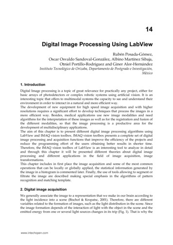
Image EnhancementPoint OperationsGrey-Scale MappingHistogram ModelingFigure 11(a) shows the histogram specified version of the image in Figure1(a) for a specified histogram in Figure 11(b) which is 1/2 cycle of asinewave. The histogram of the resultant image in Figure 11(a) is givenin Figure 11(c) which is similar in shape to the specified desired in Figure11(b). Visual comparison of the image in Figure 11(a) with those inFigure 10(a) shows much better enhancement without introducing anyundesirable artifacts.(a)(b)M.R. AzimiDigital Image Processing
Image EnhancementPoint OperationsGrey-Scale Mapping(c)Figure 11M.R. AzimiDigital Image ProcessingHistogram Modeling
Image EnhancementPoint OperationsGrey-Scale MappingHistogram ModelingExample:Histogram of a continuous image,X, is given by hX (x) Ae x wherex [0, b] and A is a normalization factor. We would like to map this2image to a new image, Y , with the desired histogram hY (y) Bye ywith range of values y [0, b] and B is the normalization factor. Find thetransformation function y T (x) that accomplishes this task.Solution:This is histogram specification problem. First, equalize both images.Z xA1Ae α dα (1 e x )w f (x) PX (x) AR1 0AR1Rbwhere AR1 is area under hX (x) i.e. AR1 A 0 e α dα A(1 e b ).Thus,(1 e x )w f (x) (1 e b )For other imageZ y21z g(y) PY (y) Bαe α dαAR2 0M.R. AzimiDigital Image Processing
Image EnhancementPoint OperationsGrey-Scale MappingHistogram ModelingLet α2 β thenZ y221Bz g(y) Be β dβ (1 e y )2AR2 02AR2R b22where AR2 B2 0 e β dβ B2 (1 e b ). Thus,2z g(y) (1 e y )(1 e b2 )Now, we should have w z which gives y T (x) g 1 (f (x)) ors1y ln1 z(1 e b2 )But using z w (1 e x )(1 e b )we getvuuy tln1 M.R. Azimi1(1 e x )(1 e b2 )(1 e b )Digital Image Processing
A similar idea can be applied to digital images. The CDF of the digital image is P X(x) Z x 0 p x( )d KX 1 k 0 N k N u(x x k) where u(x) represents a unit step function. Clearly, the CDF for discrete r.v. is a stair-step function which starts from 0 and goes to its nal value of 1, since P K 1 k 0 N k N 1. M.R. Azimi Digital Image Processing