WIXLIB

4ZHOU, MERTIKOPOULOS, BAMBOS, BOYD, AND GLYNNAssumption 1. F (x, \omega ) is continuously differentiable in x for almost all \omega \in \Omega .Assumption 2. The gradient of F is uniformly bounded in L2 , i.e., \BbbE [\ \nabla F (x;\leq M 2 for some finite M \geq 0 and all x \in \scrX .\omega )\ 2\ast ]Remark 2.1. In the above, gradients are treated as elements of the dual space\scrY \equiv \scrV \ast of \scrV . We also note that \nabla F (x; \omega ) refers to the gradient of F (x; \omega ) withrespect to x; since \Omega is not assumed to carry a differential structure, there is nodanger of confusion.Assumption 1 is a token regularity assumption which can be relaxed to account fornonsmooth objectives by using subgradient devices (as opposed to gradients). However, this would make the presentation significantly more cumbersome, so we stickwith smooth objectives throughout. Assumption 2 is also standard in the stochasticoptimization literature: it holds trivially if F is uniformly Lipschitz (another commonly used condition) and, by the dominated convergence theorem, it further impliesthat f is smooth and \nabla f (x) \nabla \BbbE [F (x; \omega )] \BbbE [\nabla F (x; \omega )] is bounded. As a result,the solution set(2.2)\scrX \ast arg min fof (Opt) is closed and nonempty (by the compactness of \scrX and the continuity of f ).We briefly discuss below two important examples of (Opt).Example 2.1 (distributed optimization). An important special case of (Opt) withhigh relevance to statistical inference, signal processing, and machine learning is whenf is of the special form(2.3)f (x) N1 \sumfi (x)N i 1for some family of functions (or training samples) fi : \scrX \rightarrow \BbbR , i 1, . . . , N . As anexample, this setup corresponds to empirical risk minimization with uniform weights,the sample index i being drawn with uniform probability from \{ 1, . . . , N \} .Example 2.2 (noisy gradient measurements). Another widely studied instance of(Opt) is when(2.4)F (x; U ) f (x) \langle U, x\ranglefor some random vector U such that \BbbE [U ] 0 and \BbbE [\ U \ 2\ast ] \infty . This gives\nabla F (x; U ) \nabla f (x) U , so (Opt) can be seen here as a model for deterministicoptimization problems with noisy gradient measurements.2.2. Variational coherence. We are now in a position to define the class ofvariationally coherent problems.Definition 2.1. We say that (Opt) is variationally coherent if(VC)\langle \nabla f (x), x - x\ast \rangle \geq 0for all x \in \scrX , x\ast \in \scrX \ast ,and there exists some x\ast \in \scrX \ast such that equality holds in (VC) only if x \in \scrX \ast .In words, (VC) states that solutions of (Opt) can be harvested by solving a(Minty) variational inequality---hence the term variational coherence."" To the bestof our knowledge, the closest analogue to this condition first appeared in the classical

ON THE CONVERGENCE OF MIRROR DESCENT5paper of Bottou [5] on online learning and stochastic approximation algorithms, butwith the added assumptions that (a) the problem (Opt) admits a unique solution x\astand (b) an extra positivity requirement for \langle \nabla f (x), x - x\ast \rangle in punctured neighborhoodsof x\ast . In the context of variational inequalities, a closely related variant of (VC) hasbeen used to establish the convergence of extragradient methods [14, 44] and SGD [19]in (Stampacchia) variational inequalities with a unique solution. By contrast, thereis no uniqueness requirement in (VC), an aspect of the definition which we examinein more detail below.We should also note that, as stated, (VC) is a nonrandom requirement for f soit applies equally well to deterministic optimization problems. Alternatively, by thedominated convergence theorem, (VC) can be written equivalently as\BbbE [\langle \nabla F (x; \omega ), x - x\ast \rangle ] \geq 0,(2.5)so it can be interpreted as saying that F is variationally coherent on average,""without any individual realization thereof satisfying (VC). Both interpretations willcome in handy later on.All in all, the notion of variational coherence will play a central role in our paperso a few examples are in order.Example 2.3 (convex programming). If f is convex, \nabla f is monotone [38] in thesense that(2.6)\langle \nabla f (x) - \nabla f (x\prime ), x - x\prime \rangle \geq 0for all x, x\prime \in \scrX .By the first-order optimality conditions for f , it follows that \langle f (x\ast ), x - x\ast \rangle \geq 0 forall x \in \scrX . Hence, by monotonicity, we get(2.7)\langle \nabla f (x), x - x\ast \rangle \geq \langle \nabla f (x\ast ), x - x\ast \rangle \geq 0for all x \in \scrX , x\ast \in \scrX \ast .By convexity, it further follows that \langle \nabla f (x), x - x\ast \rangle 0 whenever x\ast \in \scrX \ast andx \in \scrX \setminus \scrX \ast , so equality holds in (2.7) if and only if x \in \scrX \ast . This shows that convexprograms automatically satisfy (VC).Example 2.4 (quasi-convex problems). More generally, the above analysis alsoextends to quasi-convex objectives, i.e., when(QC)f (x\prime ) \leq f (x) \Rightarrow \langle \nabla f (x), x\prime - x\rangle \leq 0for all x, x\prime \in \scrX [6]. In this case, we have the following.Proposition 2.2. Suppose that f is quasi-convex and nondegenerate, i.e.,(2.8)\langle \nabla f (x), z\rangle \not 0for all nonzero z \in TC(x), x \in \scrX \setminus \scrX \ast .Then, f is variationally coherent.Remark 2.2. The nondegeneracy condition (2.8) is generic in that it is satisfiedby every quasi-convex function after an arbitrarily small perturbation leaving its minimum set unchanged. In particular, it is automatically satisfied if f is convex orpseudoconvex.Proof. Take some x\ast \in \scrX \ast and x \in \scrX . Then, letting x\prime x\ast in (QC), we readilyobtain \langle \nabla f (x), x - x\ast \rangle \geq 0 for all x \in \scrX , x\ast \in \scrX \ast . Furthermore, if x \in/ \scrX \ast but\ast\langle \nabla f (x), x - x \rangle 0, the gradient nondegeneracy condition (2.8) would be violated,implying in turn that, for any x\ast \in \scrX \ast , we have \langle \nabla f (x), x - x\ast \rangle 0 only if x \in \scrX \ast .This shows that f satisfies (VC).

6ZHOU, MERTIKOPOULOS, BAMBOS, BOYD, AND GLYNNExample 2.5 (beyond quasi-convexity). A simple example of a function that isvariationally coherent without even being quasi-convex is(2.9)f (x) 2d\sum\surd1 xi ,x \in [0, 1]d .i 1When d \geq 2, it is easy to see f is not quasi-convex:instance, taking d 2,\surd for \surdx (0, 1), and x\prime (1, 0) yields f (x/2 x\prime /2) 2 6 2 2 max\{ f (x), f (x\prime )\} ,so f is not quasi-convex. On the other hand, to estabilish (VC), simply note that\surd\sum d\scrX \ast \{ 0\} and \langle \nabla f (x), x - 0\rangle i 1 xi / 1 xi 0 for all x \in [0, 1]d \setminus \{ 0\} .Example 2.6 (a weaker version of coherence). Consider the functiond(2.10)f (x) 1 \prod 2x ,2 i 1 ix \in [ - 1, 1]d .By inspection, it is easy to see that the minimum set of f is \scrX \ast \{ x\ast \in [ - 1, 1]d :x\ast i 0 for at least one i 1, . . . , d\} .1 Since \scrX \ast is not convex for d \geq 2, f is notquasi-convex. On the other hand, we have \nabla f (x) 2f (x) \cdot (1/x1 , . . . , 1/xd ), so\langle \nabla f (x), x - 0\rangle \geq 0 for all x \in [ - 1, 1]d with equality only if x \in \scrX \ast . Moreover, for anyx\ast \in \scrX \ast and all x \in \scrX sufficiently close to x\ast , we have\right]\left[\biggr]d \biggl[\ast\ast\sum\sumxix(2.11)\geq 0.1 - i 2f (x) d -\langle \nabla f (x), x - x\ast \rangle 2f (x)xxii\asti 1i:xi \not 0We thus conclude that f satisfies the following weaker version of (VC).Definition 2.3. We say that f : \scrX \rightarrow \BbbR is weakly coherent if the following conditions are satisfied:(a) There exists some p \in \scrX \ast such that \langle \nabla f (x), x - p\rangle \geq 0 with equality only ifx \in \scrX \ast .(b) For all x\ast \in \scrX \ast , \langle \nabla f (x), x - x\ast \rangle \geq 0 whenever x is close enough to x\ast .Our analysis also applies to problems satisfying these less stringent requirements,in which case the minimum set \scrX \ast arg min f of f need not even be convex.2 Forsimplicity, we will first work with Definition 2.1 and relegate these considerations tosection 5.2.3. Stochastic mirror descent. To solve (Opt), we will focus on the SMDfamily of algorithms, a class of first-order methods pioneered by Nemirovski and Yudin[32] and studied further by Beck and Teboulle [3], Nesterov [34], Lan, Nemirovski, andShapiro [24], and many others. Referring to [8, 40] for an overview, the specific variantof SMD that we consider here is usually referred to as dual averaging [28, 34, 45] orlazy mirror descent [40].The main idea of the method is as follows: At each iteration, the algorithmtakes as input an i.i.d. sample of the gradient of F at the algorithm's current state.Subsequently, the method takes a step along this stochastic gradient in the dual space1 Linear combinations of functions of this type play an important role in training deep learningmodels---and, in particular, generative adversarial network [17].2 Obviously, Definitions 2.1 and 2.3 coincide if \scrX \ast is a singleton. This highlights the intricaciesthat arise in problems that do not admit a unique solution.

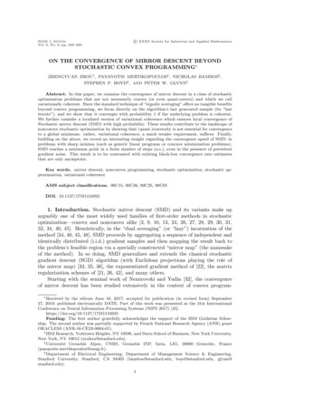
ON THE CONVERGENCE OF MIRROR DESCENT7\scrY \equiv \scrV \ast of \scrV (where gradients live), the result is mirrored"" back to the problem'sfeasible region \scrX , and the process repeats. Formally, this gives rise to the recursionXn Q(Yn ),(SMD)Yn 1 Yn - \gamma n \nabla F (Xn ; \omega n ),where1. n 1, 2, . . . denotes the algorithm's running counter,2. Yn \in \scrY is a score variable that aggregates gradient steps up to stage n,3. Q : \scrY \rightarrow \scrX is the mirror map that outputs a solution candidate Xn \in \scrX as afunction of the score variable Yn \in \scrV \ast ,4. \omega n \in \Omega is a sequence of i.i.d. samples,35. \gamma n 0 is the algorithm's step-size sequence, assumed in what follows tosatisfy the Robbins--Monro summability condition\infty\sum(2.12)\gamma n2 \inftyandn 1\infty\sum\gamma n \infty .n 1For a schematic illustration and a pseudocode implementation of (SMD), see Figure 1and Algorithm 1, respectively.Y1- \gamma 1 \nabla F (X1 ; \omega 1 )- \gamma 2 \nabla F (X2 ; \omega 2 )\scrY \scrV \astY2Y3QQQQX3\scrX \subseteq \scrVX1X2Fig. 1. Schematic representation of SMD (Algorithm 1).Algorithm 1 Stochastic mirror descent.Require: mirror map Q : \scrY \rightarrow \scrX ; step-size sequence \gamma n 01: choose Y \in \scrY \equiv \scrV \ast\# initialization2: for n 1, 2, . . . do3:set X \leftarrow Q(Y )\# set state4:draw \omega \in \Omega\# gradient sample5:get v\ - \nabla F (X; \omega )\# get oracle feedback6:set Y \leftarrow Y \gamma n v\ \# update score variable7: end for8: return X\# output3 The indexing convention for \omega means that Y and X are predictable relative to the naturalnnnfiltration \scrF n \sigma (\omega 1 , . . . , \omega n ) of \omega n , i.e., Yn 1 and Xn 1 are both \scrF n -measurable. To this history,we also attach the trivial \sigma -algebra as \scrF 0 for completeness.

8ZHOU, MERTIKOPOULOS, BAMBOS, BOYD, AND GLYNNIn more detail, the algorithm's mirror map Q : \scrY \rightarrow \scrX is defined as(2.13)Q(y) arg max\{ \langle y , x\rangle - h(x)\} ,x\in \scrXwhere the regularizer (or penalty function) h : \scrX \rightarrow \BbbR is assumed to be continuousand strongly convex on \scrX , i.e., there exists some K 0 such that(2.14)h(\tau x (1 - \tau )x\prime ) \leq \tau h(x) (1 - \tau )h(x\prime ) - 12 K\tau (1 - \tau )\ x\prime - x\ 2for all x, x\prime \in \scrX and all \tau \in [0, 1]. The mapping Q : \scrV \ast \rightarrow \scrX defined by (2.13) isthen called the mirror map induced by h. For concreteness, we present below somewell-known examples of regularizers and mirror maps.Example 2.7 (Euclidean regularization). Let h(x) 21 \ x\ 22 . Then, h is 1-stronglyconvex with respect to the Euclidean norm \ \cdot \ 2 , and the induced mirror map is theclosest point projection\bigl\{\bigr\}\Pi (y) arg max \langle y , x\rangle - 21 \ x\ 22 arg min \ y - x\ 22 .(2.15)x\in \scrXx\in \scrXThe resulting descent algorithm is known in the literature as (lazy) SGD and we studyit in detail in section 6. For future reference, we also note that h is differentiablethroughout \scrX and \Pi is surjective (i.e., im \Pi \scrX ).\sum dExample 2.8 (entropic regularization). Let \Delta \{ x \in \BbbR d : i 1 xi 1\} denotethe unit simplex of \BbbR d . A widely used regularizer in this setting is the (negative) Gibbs\sum dentropy h(x) i 1 xi log xi : this regularizer is 1-strongly convex with respect to1the L -norm and a straightforward calculation shows that the induced mirror map is(2.16)\Lambda (y) \sum di 11exp(yi )(exp(y1 ), . . . , exp(yd )).This example is known as entropic regularization and the resulting mirror descentalgorithm has been studied extensively in the context of linear programming, onlinelearning, and game theory [1, 40]. For posterity, we also note that h is differentiableonly on the relative interior \Delta \circ of \Delta and im \Lambda \Delta \circ (i.e., \Lambda is essentially"" surjective).2.4. Overview of main results. To motivate the analysis to follow, we providebelow a brief overview of our main results:\bullet Global convergence: If (Opt) is variationally coherent, the last iterate Xn of(SMD) converges to a global minimizer of f with probability 1.\bullet Local convergence: If x\ast is a locally coherent minimum point of f (a notionintroduced in section 5), the last iterate Xn of (SMD) converges locally to x\astwith high probability.\bullet Sharp minima: If Q is surjective and x\ast is a sharp minimum of f (a fundamental notion due to Polyak which we discuss in section 6), Xn reaches x\ast ina finite number of iterations (a.s.).3. Main tools and first results. As a stepping stone to analyze the long-termbehavior of (SMD), we derive in this section a recurrence result which is interestingin its own right. Specifically, we show that if (Opt) is coherent, then, with probability1, Xn visits any neighborhood of \scrX \ast infinitely often; as a corollary, there exists a(random) subsequence Xnk of Xn that converges to arg min f (a.s.). In what follows,our goal will be to state this result formally and to introduce the analytic machineryused for its proof (as well as the analysis of the subsequent sections).

ON THE CONVERGENCE OF MIRROR DESCENT93.1. The Fenchel coupling. The first key ingredient of our analysis will be theFenchel coupling, a primal-dual variant of the Bregman divergence [7] that plays therole of an energy function for (SMD).Definition 3.1. Let h : \scrX \rightarrow \BbbR be a regularizer on \scrX . The induced Fenchelcoupling F (p, y) between a base point p \in \scrX and a dual vector y \in \scrY is defined asF (p, y) h(p) h\ast (y) - \langle y , p\rangle ,(3.1)where h\ast (y) maxx\in \scrX \{ \langle y , x\rangle - h(x)\} denotes the convex conjugate of h.By Fenchel's inequality (the namesake of the Fenchel coupling), we have h(p) h\ast (y) - \langle y , p\rangle \geq 0 with equality if and only if p Q(y). As such, F (p, y) can beseen as a (typically asymmetric) distance measure"" between p \in \scrX and y \in \scrY . Thefollowing lemma quantifies some basic properties of this coupling.Lemma 3.2. Let h be a K-strongly convex regularizer on \scrX . Then, for all p \in \scrXand all y, y \prime \in \scrY , we haveK\ Q(y) - p\ 2 ,2(3.2a)(a) F (p, y) \geq(3.2b)(b) F (p, y \prime ) \leq F (p, y) \langle y \prime - y, Q(y) - p\rangle 1\ y \prime - y\ 2\ast .2KLemma 3.2 (which we prove in Appendix B) shows that Q(yn ) \rightarrow p wheneverF (p, yn ) \rightarrow 0, so the Fenchel coupling can be used to test the convergence of theprimal sequence xn Q(yn ) to a given base point p \in \scrX . For technical reasons, itwill be convenient to also make the converse assumption.Assumption 3. F (p, yn ) \rightarrow 0 whenever Q(yn ) \rightarrow p.Assumption 3 can be seen as a reciprocity condition"": essentially, it meansthat the sublevel sets of F (p, \cdot ) are mapped under Q to neighborhoods of p in \scrX(cf. Appendix B). In this way, Assumption 3 can be seen as a primal-dual analogueof the reciprocity conditions for the Bregman divergence that are widely used inthe literature on proximal and forward-backward methods [9, 23]. Most commonregularizers satisfy this technical requirement (including the Euclidean and entropicregularizers of Examples 2.7 and 2.8, respectively).3.2. Main recurrence result. To state our recurrence result, we require onelast piece of notation pertaining to measuring distances in \scrX .Definition 3.3. Let \scrC be a subset of \scrX .1. The distance between \scrC and x \in \scrX is defined as dist(\scrC , x) inf x\prime \in \scrC \ x\prime - x\ ,and the corresponding \varepsilon -neighborhood of \scrC is(3.3a)\BbbB (\scrC , \varepsilon ) \{ x \in \scrX : dist(\scrC , x) \varepsilon \} .2. The (setwise) Fenchel coupling between \scrC and y \in \scrY is defined as F (\scrC , y) inf x\in \scrC F (x, y), and the corresponding Fenchel \delta -zone of \scrC under h is(3.3b)\BbbB F (\scrC , \delta ) \{ x \in \scrX : x Q(y) for some y \in \scrY with F (\scrC , y) \delta \} .We then have the following recurrence result for variationally coherent problems.Proposition 3.4. Fix some \varepsilon 0 and \delta 0. If (Opt) is variationally coherentand Assumptions 1--3 hold, the (random) iterates Xn of Algorithm 1 enter \BbbB (\scrX \ast , \varepsilon )and \BbbB F (\scrX \ast , \delta ) infinitely many times (a.s.). pag

the problem's feasible region via a specially constructed mirror map"" (the namesake of the method). In so doing, SMD generalizes and extends the classical stochastic gradient descent (SGD) algorithm (with Euclidean projections playing the role of the mirror map) [33, 35, 36], the exponentiated gradient method of [22], the matrix