Transcription
Tropical geometry and mirror symmetryMark GrossUCSD Mathematics, 9500 Gilman Drive, La Jolla, CA 92093-0112E-mail address: mgross@math.ucsd.edu
1991 Mathematics Subject Classification. 14T05, 14M25, 14N35, 14J32, 14J33,52B20Key words and phrases. Mirror symmetry, Tropical geometryAbstract. This monograph, based on lectures given at the NSF-CBMS conference on Tropical Geometry and Mirror Symmetry at Kansas State University, aims to present a snapshot of ideas being developed by Gross and Siebertto understand mirror symmetry via tropical geometry.In this program, there are three worlds. The first part of the book presentsthese three linked realms: tropical geometry, in which geometric objects arepiecewise linear objects; the A- and B-models of mirror symmetry (GromovWitten theory and period integrals respectively); and log geometry. Log geometry is used to go between the world of tropical geometry, on the one hand,and the world of the A- and B-models, on the other.Next, one complete example is given in depth, namely mirror symmetryfor P2 . Following Siebert and Nishinou, a complete proof of Mikhalkin’s tropical curve counting theorem is given for toric surfaces. Gross’s mirror result forP2 showing how period integrals can be computed directly in terms of tropicalgeometry is then given.Finally, the book ends with a survey of the Gross-Siebert program in theCalabi-Yau case. A complete proof of the correspondence theorem betweenaffine K3 surfaces and degenerations of K3 surfaces is given, a special caseof the correspondence theorem for Calabi-Yau varieties proved by Gross andSiebert in general and proved for K3 surfaces by Kontsevich and Soibelman.
“Maybe the tropics,” somebody, probably the General said, “butnever the Polar Region, it’s too white, too mathematical upthere.”—Thomas Pynchon, Against the Day.
ContentsPrefaceixIntroductionxiPart 1.1The three worldsChapter 1. The tropics1.1. Tropical hypersurfaces1.2. Some background on fans1.3. Parameterized tropical curves1.4. Affine manifolds with singularities1.5. The discrete Legendre transform1.6. Tropical curves on tropical surfaces1.7. References and further reading33111319273032Chapter 2. The A- and B-models2.1. The A-model2.2. The B-model2.3. References and further reading33336789Chapter 3. Log geometry3.1. A brief review of toric geometry3.2. Log schemes3.3. Log derivations and differentials3.4. Log deformation theory3.5. The twisted de Rham complex revisited3.6. References and further readingPart 2.Example: P2 .919298112117126129131Chapter 4. Mikhalkin’s curve counting formula4.1. The statement and outline of the proof4.2. Log world tropical world4.3. Tropical world log world4.4. Classical world log world4.5. Log world classical world4.6. The end of the proof4.7. References and further reading133133138143157165169171Chapter 5. Period integrals5.1. The perturbed Landau-Ginzburg potential173173vii
viiiCONTENTS5.2.5.3.5.4.5.5.5.6.Part 3.Tropical descendent invariantsThe main B-model statementDeforming Q and P1 , . . . , PkEvaluation of the period integralsReferences and further reading179187192222244The Gross-Siebert program245Chapter 6. The program and two-dimensional results6.1. The program6.2. From integral tropical manifolds to degenerations in dimension two6.3. Achieving compatibility: The tropical vertex group6.4. Remarks and generalizations6.5. References and further reading247247255290305306Bibliography307Index of Symbols313General Index315
PrefaceThe NSF-CBMS conference on Tropical Geometry and Mirror Symmetry washeld at Kansas State University during the period December 13–17, 2008. It wasorganized by Ricardo Castaño-Bernard, Yan Soibelman, and Ilia Zharkov. Duringthis time, I gave ten hours of lectures. In addition, talks were given by M. Abouzaid,K.-W. Chan, C. Doran, K. Fukaya, I. Itenberg, L. Katzarkov, A. Mavlyutov, D.Morrison, Y.-G. Oh, T. Pantev, B. Siebert, and B. Young.My talks were meant to give a snapshot of a long-term program currentlybeing carried out with Bernd Siebert aimed at achieving a fundamental conceptualunderstanding of mirror symmetry. Tropical geometry emerges naturally in thisprogram, so in the lectures I took a rather ahistorical point of view. Starting withthe tropical semi-ring, I developed tropical geometry and explained Mikhalkin’stropical curve-counting formulas, outlining the proof given by Nishinou and Siebert.I then explained my recent work in connecting this to the mirror side. Finally,I sketched the ideas behind recent work by myself and Siebert on constructingdegenerations of Calabi-Yau manifolds from affine manifolds with singularities.This monograph follows the structure of the lectures closely, filling in many details which were not given there. Like the lectures, this monograph only representsa snapshot of an evolving program, but I hope it will be useful to those who maywish to become involved in this program.NSF grant DMS-0735319 provided support both for the conference and for thisbook.Mark Gross, La Jolla, 2010ix
IntroductionThe early history of mirror symmetry has been told many times; we will onlysummarize it briefly here. The story begins with the introduction of Calabi-Yaucompactifications in string theory in 1985 [11]. The idea is that, since superstringtheory requires a ten-dimensional space-time, one reconciles this with the observeduniverse by requiring (at least locally) that space-time take the formR1,3 X,where R1,3 is usual Minkowski space-time and X is a very small six-dimensionalRiemannian manifold. The desire for the theory to preserve the supersymmetryof superstring theory then leads to the requirement that X have SU(3) holonomy,i.e., be a Calabi-Yau manifold. Thus string theory entered the realm of algebraicgeometry, as any non-singular projective threefold with trivial canonical bundlecarries a metric with SU(3) holonomy, thanks to Yau’s proof of the Calabi conjecture[113].This generated an industry in the string theory community devoted to producing large lists of examples of Calabi-Yau threefolds and computing their invariants,the most basic of which are the Hodge numbers h1,1 and h1,2 .In 1989, a rather surprising observation came out of this work. Candelas,Lynker and Schimmrigk [12] provided a list of Calabi-Yau hypersurfaces in weightedprojective space which exhibited an obvious symmetry: if there was a Calabi-Yauthreefold with Hodge numbers given by a pair (h1,1 , h1,2 ), then there was often alsoone with Hodge numbers given by the pair (h1,2 , h1,1 ). Independently, guided bycertain observations in conformal field theory, Greene and Plesser [36] studied thequintic threefold and its mirror partner. If we let Xψ be the solution set in P4 ofthe equationx50 · · · x54 ψx0 x1 x2 x3 x4 0for ψ C, then for most ψ, Xψ is a non-singular quintic threefold, and as such, hasHodge numbersh1,1 (Xψ ) 1, h1,2 (Xψ ) 101.On the other hand, the groupG acts diagonally on P4 , viaQ4{(a0 , . . . , a4 ) ai µ5 , i 0 ai 1}{(a, a, a, a, a) a µ5 }(x0 , . . . , x4 ) 7 (a0 x0 , . . . , a4 x4 ).Here µ5 is the group of fifth roots of unity. This action restricts to an action onXψ , and the quotient Xψ /G is highly singular. However, these singularities can bexi
xiiINTRODUCTIONresolved via a proper birational morphism X̌ψ Xψ /G with X̌ψ a new Calabi-Yauthreefold with Hodge numbersh1,1 (X̌ψ ) 101,h1,2 (X̌ψ ) 1.These examples were already a surprise to mathematicians, since at the time veryfew examples of Calabi-Yau threefolds with positive Euler characteristic were known(the Euler characteristic coinciding with 2(h1,1 h1,2 )).Much more spectacular were the results of Candelas, de la Ossa, Green andParkes [10]. Guided by string theory and path integral calculations, Candelas etal. conjectured that certain period calculations on the family X̌ψ parameterized byψ would yield predictions for numbers of rational curves on the quintic threefold.They carried out these calculations, finding agreement with the known numbers ofrational curves up to degree 3. We omit any details of these calculations here, asthey have been exposited in many places, see e.g., [43]. This agreement was verysurprising to the mathematical community, as these numbers become increasinglydifficult to compute as the degree increases. The number of lines, 2875, was knownin the 19th century, the number of conics, 609250, was computed only in 1986by Sheldon Katz [66], and the number of twisted cubics, 317206375, was onlycomputed in 1990 by Ellingsrud and Strømme [22].Throughout the history of mathematics, physics has been an important sourceof interesting problems and mathematical phenomena. Some of the interestingmathematics that arises from physics tends to be a one-off — an interesting andunexpected formula, say, which once verified mathematically loses interest. Othercontributions from physics have led to powerful new structures and theories whichcontinue to provide interesting and exciting new results. I like to believe that mirrorsymmetry is one of the latter types of subjects.The conjecture raised by Candelas et al., along with related work, led to thestudy of Gromov-Witten invariants (defining precisely what we mean by “the number of rational curves”) and quantum cohomology, a way of deforming the usual cupproduct on cohomology using Gromov-Witten invariants. This remains an activefield of research, and by 1996, the theory was sufficiently developed to allow proofsof the mirror symmetry formula for the quintic by Givental [34], Lian, Liu and Yau[75] and subsequently others, with the proofs getting simpler over time.Concerning mirror symmetry, Batyrev [6] and Batyrev-Borisov [7] gave verygeneral constructions of mirror pairs of Calabi-Yau manifolds occurring as completeintersections in toric varieties. In 1994, Maxim Kontsevich [68] made his fundamental Homological Mirror Symmetry conjecture, a profound effort to explain therelationship between a Calabi-Yau manifold and its mirror in terms of categorytheory.In 1996, Strominger, Yau and Zaslow proposed a conjecture, [108], now referredto as the SYZ conjecture, suggesting a much more concrete geometric relationshipbetween mirror pairs; namely, mirror pairs should carry dual special Lagrangianfibrations. This suggested a very explicit relationship between a Calabi-Yau manifold and its mirror, and initial work in this direction by myself [37, 38, 39] andWei-Dong Ruan [97, 98, 99] indicates the conjecture works at a topological level.However, to date, the analytic problems involved in proving a full-strength version of the SYZ conjecture remain insurmountable. Furthermore, while a proof ofthe SYZ conjecture would be of great interest, a proof alone will not explain thefiner aspects of mirror symmetry. Nevertheless, the SYZ conjecture has motivated
INTRODUCTIONxiiiseveral points of view which appear to be yielding new insights into mirror symmetry: notably, the rigid analytic program initiated by Kontsevich and Soibelmanin [69, 70] and the program developed by Siebert and myself using log geometry,[47, 48, 51, 49].These ideas which grew out of the SYZ conjecture focus on the base of theSYZ fibration; even though we do not know an SYZ fibration exists, we have agood guess as to what these bases look like. In particular, they should be affinemanifolds, i.e., real manifolds with an atlas whose transition maps are affine lineartransformations. In general, these manifolds have a singular locus, a subset notcarrying such an affine structure. It is not difficult to write down examples of suchmanifolds which we expect to correspond, say, to hypersurfaces in toric varieties.More precisely,Definition 0.1. An affine manifold B is a real manifold with an atlas ofcoordinate charts{ψi : Ui Rn }with ψi ψj 1 Aff(Rn ), the affine linear group of Rn . We say B is tropical(respectively integral ) if ψi ψj 1 Rn GLn (Z) Aff(Rn ) (respectively ψi ψj 1 Aff(Zn ), the affine linear group of Zn ).In the tropical case, the linear part of each coordinate transformation is integral,and in the integral case, both the translational and linear parts are integral.Given a tropical manifold B, we have a family of lattices Λ TB generatedlocally by / y1 , . . . , / yn, where y1 , . . . , yn are affine coordinates. The conditionon transition maps guarantees that this is well-defined. Dually, we have a family oflattices Λ̌ TB generated by dy1 , . . . , dyn , and then we get two torus bundlesf : X(B) Bfˇ : X̌(B) BwithX(B) TB /Λ,X̌(B) TB /Λ.Now X(B) carries a natural complex structure. Sections of Λ are flat sections ofa connection on TB , and the horizontal and vertical tangent spaces of this connectionare canonically isomorphic. Thus we can write down an almost complex structureJ which interchanges these two spaces, with an appropriate sign-change so thatJ 2 id. It is easy to see that this almost complex structure on TB is integrableand descends to X(B).On the other hand, TB carries a canonical symplectic form which descends toX̌(B), so X̌(B) is canonically a symplectic manifold.We can think of X(B) and X̌(B) as forming a mirror pair; this is a simpleversion of the SYZ conjecture. In this simple situation, however, there are fewinteresting compact examples, in the Kähler case being limited to the possibilitythat B Rn /Γ for a lattice Γ (shown in [15]). Nevertheless, we can take thissimple case as motivation, and ask some basic questions:(1) What geometric structures on B correspond to geometric structures ofinterest on X(B) and X̌(B)?(2) If we want more interesting examples, we need to allow B to have singularities, i.e., have a tropical affine structure on an open set B0 B with
xivINTRODUCTIONB \ B0 relatively small (e.g., codimension at least two). How do we dealwith this?By 2000, it was certainly clear to many of the researchers in the field thatholomorphic curves in X(B) should correspond to certain sorts of piecewise lineargraphs in B. Kontsevich suggested the possibility that one might be able to actuallycarry out a curve count by counting these graphs. In 2002, Mikhalkin [79, 80]announced that this was indeed possible, introducing and proving curve-countingformulas for toric surfaces. This was the first evidence that one could really computeinvariants using these piecewise linear graphs. For historical reasons which will beexplained in Chapter 1, Mikhalkin called these piecewise linear graphs “tropicalcurves,” introducing the word “tropical” into the field.This brings us to the following picture. Mirror symmetry involves a relationshipbetween two different types of geometry, usually called the A-model and the Bmodel. The A-model involves symplectic geometry, which is the natural categoryin which to discuss such things as Gromov-Witten invariants, while the B-modelinvolves complex geometry, where one can discuss such things as period integrals.This leads us to the following conceptual framework for mirror symmetry:A-modelB-modelTropicalgeometryHere, we wish to explain mirror symmetry by identifying what we shall refer toas tropical structures in B which can be interpreted as geometric structures in theA- and B-models. However, the interpretations in the A- and B-models shouldbe different, i.e., mirror, so that the fact that these structures are given by thesame tropical structures then gives a conceptual explanation for mirror symmetry. For the most well-known aspect of mirror symmetry, namely the enumerationof rational curves, the hope should be that tropical curves on B correspond to(pseudo)-holomorphic curves in the A-model and corrections to period calculationsin the B-model.The main idea of my program with Siebert is to try to understand how to gobetween the tropical world and the A- and B-models by passing through anotherworld, the world of log geometry. One can view log geometry as half-way betweentropical geometry and classical geometry:
INTRODUCTIONA-modellog geometryxvB-modelTropicalgeometryAs this program with Siebert is ongoing, with much work still to be done, mylectures at the CBMS regional conference in Manhattan, Kansas were intended togive a snapshot of the current state of this program. This monograph closely followsthe outline of those lectures. The basic goal is threefold.First, I wish to explain explicitly, at least in special cases, all the worlds suggested in the above diagram: the tropical world, the “classical” world of the A- andB-model, and log geometry.Second, I would like to explain one very concrete case where the full picturehas been worked out for both the A- and B-models. This is the case of P2 . For theA-model, curve counting is the result of Mikhalkin, and here I will give a proof ofhis result adapted from a more general result of Nishinou and Siebert [86], as thatapproach is more in keeping with the philosophy of the program. For the B-model,I will explain my own recent work [42] which shows how period integrals extracttropical information.Third, I wish to survey some of the results obtained by Siebert and myself inthe Calabi-Yau case, outlining how this approach can be expected to yield a proofof mirror symmetry. While for P2 I give complete details, this third part is intendedto be more of a guide for reading the original papers, which unfortunately are quitelong and technical. I hope to at least convey an intuition for this approach.I will take a very ahistorical approach to all of this, starting with the basics oftropical geometry and working backwards, showing how a study of tropical geometry can lead naturally to other concepts which first arose in the study of mirrorsymmetry. In a way, this may be natural. To paraphrase Witten’s statement aboutstring theory, mirror symmetry often seems like a piece of twenty-first century mathematics which fell into the twentieth century. Its initial discovery in string theoryrepresents some of the more difficult aspects of the theory. Even an explanation ofthe calculations carried out by Candelas et al. can occupy a significant portion of acourse, and the theory built up to define and compute Gromov-Witten invariants iseven more involved. On the other hand, the geometry that now seems to underpinmirror symmetry, namely tropical geometry, is very simple and requires no particular background to understand. So it makes sense to develop the discussion fromthe simplest starting point.The prerequisites of this volume include a familiarity with algebraic geometryat the level of Hartshorne’s text [57] as well as some basic differential geometry.In addition, familiarity with toric geometry will be very helpful; the text will recallmany of the basic necessary facts about toric geometry, but at least some previous experience will be useful. For a more in-depth treatment of toric geometry, I
xviINTRODUCTIONrecommend Fulton’s lecture notes [27]. We shall also, in Chapter 3, make use ofsheaves in the étale topology, which can be reviewed in [83], Chapter II. However,this use is not vital to most of the discussion here.I would like to thank many people. Foremost, I would like to thank RicardoCastaño-Bernard, Yan Soibelman, and Ilia Zharkov for organizing the NSF-CBMSconference at Kansas State University. Second, I would like to thank Bernd Siebert;the approach in this book grew out of our joint collaboration. I also thank the manypeople who answered questions and commented on the manuscript, including SeanKeel, M. Brandon Meredith, Rahul Pandharipande, D. Peter Overholser, DanielSchultheis, and Katharine Shultis.Parts of this book were written during a visit to Oxford; I thank Philip Candelasfor his hospitality during this visit. The final parts of the book were written duringthe fall of 2009 at MSRI; I thank MSRI for its financial support via a SimonsProfessorship.I would like to thank Lori Lejeune for providing the files for Figures 17, 18 and19 of Chapter 1 and Figures 7 and 8 of Chapter 6. Finally, and definitely not least,I thank Arthur Greenspoon, who generously offered to proofread this volume.Convention. Throughout this book k denotes an algebraically closed field ofcharacteristic zero. N denotes the set of natural numbers {0, 1, 2, . . .}.
Part 1The three worlds
CHAPTER 1The tropicsWe start with the simplest of the three worlds, the tropical world. Tropicalgeometry is a kind of piecewise linear combinatorial geometry which arises whenone starts to think about algebraic geometry over the so-called tropical semi-ring.This chapter will give a rather shallow introduction to the subject. We will startwith the definition of the tropical semi-ring and some elementary algebraic geometryover the tropical semi-ring. We move on to the notion of parameterized tropicalcurve, which features in Mikhalkin’s curve counting results. Next, we introduce thetype of tropical objects which arise in the Gross-Siebert program: affine manifoldswith singularities. These arise naturally if one wants to think about curve countingin Calabi-Yau manifolds. We end with a duality between such objects given by theLegendre transform.1.1. Tropical hypersurfacesWe begin with the tropical semi-ring,Rtrop (R, , ).Here R is the set of real numbers, but with addition and multiplication defined bya ba b: min(a, b): a b.Of course there is no additive inverse. This semi-ring became known as the tropicalsemi-ring in honour of the Brazilian mathematician Imre Simon. The word tropicalhas now spread rapidly.We would like to do algebraic geometry over the tropical semi-ring instead ofover a field. Of course, since there is no additive identity in this semi-ring, it is notimmediately obvious what the zero-locus of a polynomial should be. The correct,or rather, useful, intepretation is as follows. LetRtrop [x1 , . . . , xn ]denote the space of functions f : Rn R given by tropical polynomialsXai1 ,.,in xi11 · · · xinnf (x1 , . . . , xn ) (i1 ,.,in ) Snwhere S Z is a finite index set. Here all operations are in Rtrop , so this is reallythe functionnXik xk (i1 , . . . , in ) S}f (x1 , . . . , xn ) min{ai1 ,.,in k 1This is a piecewise linear function, and the tropical hypersurface defined by f ,V (f ) Rn , as a set, is the locus where f is not linear.3
41. THE TROPICSx10Figure 1. 0 (0 x1 )In order to write these formulas in a more invariant way, in what follows weshall often make use of the notationM Zn ,MR M Z R,N HomZ (M, Z),NR N Z R.We denote evaluation of n N on m M by hn, mi. We shall often use thenotion of index of an element m M \ {0}; this is the largest positive integer rsuch that there exists m′ M with rm′ m. If the index of m is 1, we say m isprimitive.With this notation, we can view a tropical function as a map f : MR Rwritten, for S N a finite set, asXf (z) an z n : min{an hn, zi n S}.n SNow V (f ) will be a union of codimension one polyhedra in Rn . Here, by apolyhedron, we mean:Definition 1.1. A polyhedron σ in MR is a finite intersection of closed halfspaces. A face of a polyhedron is a subset given by the intersection of σ with ahyperplane H such that σ is contained in a half-space with boundary H.The boundary σ of σ is the union of all proper faces of σ, and the interiorInt(σ) of σ is σ \ σ.The polyhedron σ is a lattice polyhedron if it is an intersection of half-spacesdefined over Q and all vertices of σ lie in M .A polytope is a compact polyhedron.Returning to V (f ), each codimension one polyhedron making up V (f ) separatestwo domains of linearity of f , in one of which f is given by a monomial withexponent n N and in the other by a monomial with exponent n′ N . Then theweight of this polyhedron in V (f ) is the index of n′ n. We then view V (f ) as aweighted polyhedral complex.Examples 1.2. Figures 1 through 5 give examples of two-variable tropicalpolynomials and their corresponding “zero loci.” All edges have weight 1 unlessotherwise indicated. We also indicate the monomial determining the function oneach domain of linearity and the precise position of the vertices.We now explain a simple way to see what V (f ) looks like. GivenXf an z n ,n S
1.1. TROPICAL HYPERSURFACES51x1(1, 1)x2Figure 2. 1 (0 x1 ) (0 x2 )0x1(0, 0)5 2x1( 5, 1)( 1, 1)x21 x1 x2( 1, 5)5 2x2Figure 3. 0 (0 x1 ) (0 x2 ) (1 x1 x2 ) (5 x1 x1 ) (5 x2 x2 )0x19 2x1( 9, 3)(0, 0)x2( 1, 1)( 5, 3)1 2x23 x1 x2Figure 4. 0 (0 x1 ) (0 x2 ) (3 x1 x2 ) (9 x1 x1 ) (1 x2 x2 )we consider the Newton polytope of S, S : Conv(S) NR ,
61. THE TROPICSx10(0, 0)2(1, 1)2x1 2x21 x2Figure 5. 0 (0 x1 ) (1 x2 ) (0 x1 x1 x2 x2 ) S (3, 2)(0, 1)(1, 0)(2, 0) S0123Figure 6the convex hull of S in NR . The coefficients an then define a functionϕ : S R S of the setas follows. We consider the upper convex hull S̃ {(n, an ) n S} NR R,namely S {(n, a) NR R there exists (n, a′ ) Conv(S̃) with a a′ }. We then define S }.ϕ(n) min{a R (n, a) For example, considering the univariate tropical polynomialf 1 (0 x) (0 x2 ) (2 x3 ), S as depicted in Figure 6, with the lower boundary of S beingwe get S and the graph of ϕ.This picture yields a polyhedral decomposition of S :Definition 1.3. A (lattice) polyhedral decomposition of a (lattice) polyhedron NR is a set P of (lattice) polyhedra in NR called cells such that
1.1. TROPICAL HYPERSURFACES7 S 20 1m 1m 2m 1/2 S . The right-hand pictureFigure 7. The left-hand figure is shows P̌ on the x-axis and the graph of ϕ̌.S(1) σ P σ.(2) If σ P and τ σ is a face, then τ P.(3) If σ1 , σ2 P, then σ1 σ2 is a face of both σ1 and σ2 .For a polyhedral decomposition P, denote by Pmax the subset of maximal cells ofP. We denote by P [k] the set of k-dimensional cells of P.Indeed, to get a polyhedral decomposition P of S , we just take P to be S. Athe set of images under the projection NR R NR of proper faces of polyhedral decomposition of S obtained in this way from the graph of a convexpiecewise linear function is called a regular decomposition and these decompositionsplay an important role in the combinatorics of convex polyhedra, see e.g., [32].We can now define the discrete Legendre transform of the triple ( S , P, ϕ):Definition 1.4. The discrete Legendre transform of ( S , P, ϕ) is the triple(MR , P̌, ϕ̌) where:(1)P̌ {τ̌ τ P}withτ̌ (m MR a R such that h m, ni a ϕ(n)for all n S , with equality for n τ).(2) ϕ̌(m) max{a h m, ni a ϕ(n) for all n S }.Let us explain this in a bit more detail. First, if σ Pmax , let mσ M be theslope of ϕ σ . Then in factσ̌ { mσ },as follows from the convexity of ϕ. Second, the formula in (2) is a fairly standardway of describing the Legendre transformed function ϕ̌. We think of ϕ̌(m) asobtained by taking the graph in NR R of a linear function on NR with slope m S . Theand moving it up or down until it becomes a supporting hyperplane for value of this affine linear function at 0 is then ϕ̌(m); see Figure 7. Note that ifm Int(τ̌ ), then the graph of h m, ·i ϕ̌(m) is then a supporting hyperplane for S projecting isomorphically to τ .the face of
81. THE TROPICS00Figure 8. The Newton polytope and subdivision for Figure 1.In fact, ϕ̌ can be described in a more familiar way. Note thatϕ̌(m) min{ϕ(n) hm, ni n S }.From this, it is clear that P̌max consists of the maximal domains of linearity ofϕ̌, with ϕ̌ v̌ having slope v for v a vertex (element of P [0] ) of P. Indeed, theminimum is always achieved at some vertex, and if this vertex is v, then ϕ̌(m) ϕ(v) hm, vi. Thus ϕ̌ is linear on v̌ with slope v. Furthermore, as necessarilyϕ(v) hm, vi ϕ(v ′ ) hm, v ′ i whenever m v̌, one sees that ϕ̌ is in fact given bythe tropical polynomialXϕ(n)z n .n P [0]This is not necessarily the original polynomial defining the function f . However, S are of the form (n, an ) for n P [0] S, so ϕ(n) anclearly the vertices of for n P [0] , and the tropical polynomial defining ϕ̌ is simply missing some of theterms of the original defining polynomial f . These missing terms are precisely ones S . We can see that such termsof the form an z n with (n, an ) not a vertex of S for someare irrelevant for calculating f . Indeed, if (n, an ) is not a vertex of n N S , and f (m) hm, ni an for some m MR , thenhm, ni an hm, n′ i an′for all n′ S. But then the hyperplane in NR R given by{(n′ , r) NR R hm, n′ i r hm, ni an } S which contains (n, an ), and hence must alsois a supporting hyperplane for ′ ′contain a vertex (n , an ) of S . Then f (m) coincides with hm, n′ i an′ , and hencethe term an z n was irrelevant for calculating f . Thus we seeϕ̌ f.Since the domains of linearity of ϕ̌ are the polyhedra of P̌max , we see that[τ̌ .V (f ) τ P [1]Since the 0-cells of P̌ are the cells σ̌ { mσ } for σ Pmax , it is usally easy todraw V (f ) using this description. Additionally, the weights are easily determined:for τ P [1] , the weight of τ̌ is just the affine length of τ , i.e., the index of thedifference of the endpoints of τ .To summarize, the function ϕ determines the dual decomposition P̌, whosevertices are given by slopes of ϕ, and V (f ) is the codimension one skeleton of P̌.Examples 1.5. For the examples of Figures 1 through 5, the Newton polytopesalong with their regular decomposition and values of an are given in Figures 8throught 12.
1.1. TROPICAL HYPERSURFACES9001Figure 9. The Newton polytope and subdivision for Figure 2.510050Figure 10. The Newton polytope and subdivision for Figure 3.130009Figure 11. The Newton polytope and subdivision for Figure 4.This description of V (f ) leads to an important condition known as the balancingcondition. Specifically, for each ω̌ P̌ [n 2] , a codimension two cell, let τ̌1 , . . . , τ̌k P̌ [n 1] be the cells containing it in V (f ), with weights w1 , . . . , wk . Note th
of the mirror symmetry formula for the quintic by Givental [34], Lian, Liu and Yau [75] and subsequently others, with the proofs getting simpler over time. Concerning mirror symmetry, Batyrev [6] and Batyrev-Borisov [7] gave very general constructions of mirror pairs of Calabi-Yau manifolds occurring as complete intersections in toric varieties.