WIXLIB

17Mirror DescentThe gradient descent algorithm of the previous chapter is generaland powerful: it allows us to (approximately) minimize convex functions over convex bodies. Moreover, it also works in the model ofonline convex optimization, where the convex function can vary overtime, and we want to find a low-regret strategy—one which performswell against every fixed point x .This power and broad applicability means the algorithm is notalways the best for specific classes of functions and bodies: for instance, for minimizing linear functions over the probability simplex n , we saw in §16.4.1 that the generic gradient descent algorithmdoes significantly worse than the specialized Hedge algorithm. Thissuggests asking: can we somehow change gradient descent to adapt to the“geometry” of the problem?The mirror descent framework of this section allows us to do precisely this. There are many different (and essentially equivalent) waysto explain this framework, each with its positives. We present twoof them here: the proximal point view, and the mirror map view,and only mention the others (the preconditioned or quasi-Newtongradient flow view, and the follow the regularized leader view) inpassing.17.1Mirror Descent: the Proximal Point ViewHere is a different way to arrive at the gradient descent algorithmfrom the last lecture: Indeed, we can get an expression for xt 1 byAlgorithm 15: Proximal Gradient Descent Algorithm15.115.215.3x1 starting pointfor t 1 to T doxt 1 arg minx {η ⟨ f t ( xt ), x ⟩ 12 x x t 2 }

218mirror descent: the proximal point viewsetting the gradient of the function to zero; this gives us the expressionη · f t ( x t ) ( x t 1 x t ) 0 x t 1 x t η · f t ( x t ),which matches the normal gradient descent algorithm. Moreover, theintuition for this algorithm also makes sense: if we want to minimizethe function f t ( x ), we could try to minimize its linear approximationf t ( xt ) ⟨ f t ( xt ), x xt ⟩ instead. But we should be careful not to“over-fit”: this linear approximation is good only close to the pointxt , so we could add in a penalty function (a “regularizer”) to preventus from straying too far from the point xt . This means we shouldminimize1xt 1 arg min{ f t ( xt ) ⟨ f t ( xt ), x xt ⟩ x xt 2 }x2or dropping the terms that don’t depend on x,xt 1 arg min{⟨ f t ( xt ), x ⟩ x1 x x t 2 }2(17.1)If we have a constrained problem, we can change the update step to:xt 1 arg min{η ⟨ f t ( xt ), x ⟩ x K1 x x t 2 }2(17.2)The optimality conditions are a bit more complicated now, but theyagain can show this algorithm is equivalent to projected gradientdescent from the previous chapter.Given this perspective, we can now replace the squared Euclideannorm by other distances to get different algorithms. A particularlyuseful class of distance functions are Bregman divergences, which wenow define and use.17.1.1Bregman DivergencesGiven a strictly convex function h, we can define a distance based onhow the function differs from its linear approximation:Definition 17.1. The Bregman divergence from x to y with respect tofunction h isDh (y x ) : h(y) h( x ) ⟨ h( x ), y x ⟩.The figure on the right illustrates this definition geometrically for aunivariate function h : R R. Here are a few examples:1. For the function h( x ) 21 x 2 from Rn to R, the associated Bregman divergence isDh (y x ) 21 y x 2 ,the squared Euclidean distance.Figure 17.1: Dh (y x ) for functionh : R R.

mirror descent2192. For the (un-normalized) negative entropy function h( x ) in 1 ( xi ln xi x i ), yDh (y x ) i yi ln xi yi xi .iUsing that i yi i xi 1 for y, x n gives us Dh (y x ) y i yi ln xii for x, y n : this is the Kullback-Leibler (KL) divergencebetween probability distributions.Many other interesting Bregman divergences can be defined.17.1.2Changing the Distance FunctionSince the distance function 21 x y 2 in (17.1) is a Bregman divergence, what if we replace it by a generic Bregman divergence: whatalgorithm do we get in that case? Again, let us first consider the unconstrained problem, with the update:xt 1 arg min{η ⟨ f t ( xt ), x ⟩ Dh ( x xt )}.xAgain, setting the gradient at xt 1 to zero (i.e., the optimality condition for xt 1 ) now gives:η f t ( xt ) h( xt 1 ) h( xt ) 0,or, rephrasing h ( x t 1 ) h ( x t ) η f t ( x t ) xt 1 h 1 h( xt ) η f t ( xt )Let’s consider this for our two running examples:1. When h( x ) 12 (17.3)(17.4) x 2 , the gradient h( x ) x. So we getx t 1 x t η f t ( x t ),the standard gradient descent update.2. When h( x ) i ( xi ln xi xi ), then h( x ) (ln x1 , . . . , ln xn ), so( xt 1 )i eln(xt )i η f t (xt ) ( xt )i e η f t (xt ) .Now if f t ( x ) ⟨ℓt , x ⟩, its gradient is just the vector ℓt , and we getback precisely the weights maintained by the Hedge algorithm!The same ideas also hold for constrained convex minimization:we now have to search for the minimizer within the set K. In thiscase the algorithm using negative entropy results in the same Hedgelike update, followed by scaling the point down to get a probabilityvector, thereby giving the probability values in Hedge.To summarize: this algorithm that tries to minimize the linear ap-What would be the “right” choice of hto minimize the function f ? It wouldbe h f , because adding D f ( x xt )to the linear approximation of f at xtgives us back exactly f . Of course, theupdate now requires us to minimizef ( x ), which is the original problem. Sowe should choose an h that is “similar”to f , and yet such that the update stepis tractable.

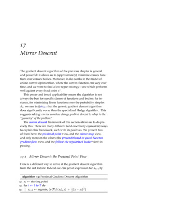
220mirror descent: the mirror map viewAlgorithm 16: Proximal Gradient Descent Algorithm16.116.216.3x1 starting pointfor t 1 to T doxt 1 arg minx K {η ⟨ f t ( xt ), x ⟩ Dh ( x xt )}proximation of the function, regularized by a Bregman distance Dh ,gives us vanilla gradient descent for one choice of h (which is goodfor quadratic-like functions over Euclidean space), and Hedge for another choice of h (which is good for linear functions over the space ofprobability distributions). Indeed, depending on how we choose thefunction, we can get different properties from this algorithm—this isthe mirror descent framework.17.2Mirror Descent: The Mirror Map ViewA different view of the mirror descent framework is the one originally presented by Nemirovski and Yudin. They observe that ingradient descent, at each step we set xt 1 xt η f t ( xt ). However,the gradient was actually defined as a linear functional on Rn andhence naturally belongs to the dual space of Rn . The fact that werepresent this functional (i.e., this covector) as a vector is a matter ofconvenience, and we should exercise care.In the vanilla gradient descent method, we were working in Rn endowed with ℓ2 -norm, and this normed space is self-dual, so it is perhaps reasonable to combine points in the primal space (the iterates xtof our algorithm) with objects in the dual space (the gradients). Butwhen working with other normed spaces, adding a covector f t ( xt )to a vector xt might not be the right thing to do. Instead, Nemirovskiand Yudin propose the following:A linear functional on vector space X isa linear map from X into its underlyingfield F.1. we map our current point xt to a point θt in the dual space using amirror map.2. Next, we take the gradient stepθ t 1 θ t η f t ( x t ).3. We map θt 1 back to a point in the primal space xt′ 1 using theinverse of the mirror map from Step 1.4. If we are in the constrained case, this point xt′ 1 might not be inthe convex feasible region K, so we to project xt′ 1 back to a “closeby” xt 1 in K.Figure 17.2: The four basic steps ineach iteration of the mirror descentalgorithm

mirror descent221The name of the process comes from thinking of the dual space as being a mirror image of the primal space. But how do we choose these mirror maps? Again, this comes down to understanding the geometryof the problem, the kinds of functions and the set K we care about,and the kinds of guarantees we want. In order to discuss these, let usdiscuss the notion of norms in some more detail.17.2.1Norms and their DualsDefinition 17.2 (Norm). A function · : Rn R is a norm if If x 0 for x Rn , then x 0; for α R and x Rn we have αx α x ; and for x, y Rn we have x y x y .The well-known ℓ p -norms for p 1 are defined byn x p : ( xi p )1/pi 1for x Rn .The ℓ -norm is given byn x : max xi i 1for x Rn .Definition 17.3 (Dual Norm). Let · be a norm. The dual norm of · is a function · defined as y : sup{⟨ x, y⟩ : x 1}.The dual norm of the ℓ2 -norm is again the ℓ2 -norm; the Euclideannorm is self-dual. The dual for the ℓ p -norm is the ℓq -norm, where1/p 1/q 1.Corollary 17.4 (Cauchy-Schwarz for General Norms). For x, y Rn ,we have ⟨ x, y⟩ x y .Proof. Assume x ̸ 0, otherwise both sides are 0. Since x/ x 1, we have ⟨ x/ x , y⟩ y .Theorem 17.5. For a finite-dimensional space with norm · , we have( · ) · .Using the notion of dual norms, we can give an alternative characterization of Lipschitz continuity for a norm · , much like Fact 16.6for Euclidean norms:Fact 17.6. For f be a differentiable function. Then f is G-Lipschitzwith respect to norm · if and only if for all x R, f ( x ) G.Figure 17.3: The unit ball in ℓ1 -norm(Green), ℓ2 -norm (Blue), and ℓ -norm(Red).

222mirror descent: the mirror map view17.2.2Defining the Mirror MapsTo define a mirror map, we first fix a norm · , and then choose adifferentiable convex function h : Rn R that is α-strongly-convexwith respect to this norm. Recall from §16.5.1 that such a functionmust satisfyh(y) h( x ) ⟨ h( x ), y x ⟩ α y x 2 .2We use two familiar examples:1. h( x ) 12 x 22 is 1-strongly convex with respect to · 2 , and2. h( x ) : in 1 xi (log xi 1) is 1-strongly convex with respect to · 1 ; the proof of this is called Pinsker’s inequality.Having fixed · and h, the mirror map isCheck out the two proofs pointed to byAryeh Kontorovich, or this proof (part1, part 2) by Madhur Tulsiani. (h) : Rn Rn .Since h is differentiable and strongly-convex, we can define the inverse map as well. This defines the mappings that we use in theNemirovski-Yudin process: we setθt h( xt )andxt′ 1 ( h) 1 (θt 1 ).For our first running example of h( x ) 21 x 2 , the gradient (andhence its inverse) is the identity map. For the (un-normalized) negative entropy example, ( h( x ))i ln xi , and hence ( h) 1 (θ )i eθi .17.2.3The Algorithm (Again)Let us formally state the algorithm again, before we state and provea theorem about it. Suppose we want to minimize a convex functionf over a convex body K Rn . We first fix a norm · on Rn andchoose a distance-generating function h : Rn R, which gives themirror map h : Rn Rn . In each iteration of the algorithm, we dothe following:(i) Map to the dual space θt h( xt ).(ii) Take a gradient step in the dual space: θt 1 θt ηt · f t ( xt ).(iii) Map θt 1 back to the primal space xt′ 1 ( h) 1 (θt 1 ).(iv) Project xt′ 1 back into the feasible region K by using the Bregmandivergence: xt 1 minx K Dh ( x xt′ 1 ). In case xt′ 1 K, e.g., inthe unconstrained case, we get xt 1 xt′ 1 .Note that the choice of h affects almost every step of this algorithm.The function h used in this way is oftencalled a distance-generating function.