WIXLIB

c J. Fessler, May 27, 2004, 13:11 (student version)4.7skim4.1.3 Existence of the Continuous-Time Fourier TransformSufficient conditions for xa (t) that ensure that the Fourier transform exists: xa (t) is absolutely integrable (over all of R). xa (t) has only a finite number of discontinuities and a finite number of maxima and minima in any finite region. xa (t) has no infinite discontinuities.Do these conditions guarantee that taking a FT of a function xa (t) and then taking the inverse FT will give you backexactly the same function xa (t)? No! Consider the function 1, t 0xa (t) 0, otherwise.Since this function (called a “null function”) has no “area,” Xa (F ) 0, so the inverse FT x̃ F 1 [X] isR simply x̃a (t) 20, whichdoes not equal xa (t) exactly! However, x and x̃ are equivalent in the L2 (R2 ) sense that kx x̃k2 xa (t) x̃a (t) dt 0,which is more than adequate for any practical problem.If we restrict attention to continuous functions xa (t), then it will be true that x F 1 [F[x]].Most physical functions are continuous, or at least do not have type of isolated points that the function x a (t) above has, so theabove mathematical subtleties need not deter our use of transform methods.We can safely restrict attention to functions xa (t) for which x F 1 [F[x]] in this course.R Lerch’s theorem: if f and g have the same Fourier transform, then f g is a null function, i.e., f (t) g(t) dt .4.2Frequency Analysis of Discrete-Time SignalsIn Ch. 2, we analyzed LTI systems using superposition. We decomposed the input signal x[n] into a train of shifted delta functions:x[n] Xck xk [n] Xk k x[k] δ[n k],Tdetermined the response to eachP shifted delta function δ[n k] hk [n], and then used linearity and time-invariance to find theoverall output signal: y[n] k x[k] h[n k] .The “shifted delta” decomposition is not the only useful choice for the “elementary” functions x k [n]. Another useful choice is thecollection of complex-exponential signals {e ωn } for various ω.We have already seen that the response of an LTI system to the input e ωn is H(ω) e ωn , where H(ω) is the frequency responseof the system.T Ch 2: xk [n] δ[n k] yk [n] h[n k]T Ch 4: xk [n] e ωk n yk [n] H(ωk ) e ωk nSo now we just need to figure out how to do the decomposition of x[n] into a weighted combination of complex-exponential signals.We begin with the case where x[n] is periodic.

c J. Fessler, May 27, 2004, 13:11 (student version)4.84.2.1The Fourier series for discrete-time periodic signalsFor a DT periodic signal, should an infinite set of frequency components be required? No, because DT frequencies aliasto the interval [ π, π].Fact: if x[n] is periodic with period N , then x[n] has the following series representation: (synthesis, inverse DTFS):x[n] N 1Xck e ωk n , where ωk k 02πk. picture of ωk ’s on [0, 2π)N(4-1)Intuition: if x[n] has period N , then x[n] has N degrees of freedom. The N ck ’s in the above decomposition express those degreesof freedom in another coordinate system.Undergrads: skim. Grads: study.Linear algebra / matrix perspectiveTo prove (4-1), one can use the fact that the N N matrix W with n, kth element Wn,k ethe elements from 0 to N 1. In fact, the columns of W are orthogonal. 2πN knis invertible, where we numberTo show that the columns are orthogonal, we first need the following simple property: Xm 0, N, 2N, . . .δ[m kN ] . otherwise N 11 X 2π nm1,N e0,N n 0k The case where m is a multiple of N is trivial, since clearly e 2πn(kN )/N e 2πnk 1 sois not a multiple of N , we can apply the finite geometric series formula:1NN 1X2πe N nm n 01NN 1 X2πe N mn 0 n1NPN 1n 01 1. For the case where m 2π N1 e N m11 11 2π 0. N 1 e 2πNmN1 e N mNow let w k and wl be two columns of the matrix W, for k, l 0, . . . , N 1. Then the inner product of these two columns ishwk , wl i N 1Xwnk (wnl ) n 0N 1X2π2πe N kn e N ln n 0n 0proving that the columns of W are orthogonal. This also proves that W0 its Hermitian transpose:W0 1 W00 1 W0 ,NN 1X2πe N (k l)n N δ[k l], 1 WNis an orthonormal matrix, so its inverse is justwhere “ ” denotes Hermitian transpose. Furthermore,0 1 111W 1 ( N W0 ) 1 W0 1 W0 W0 .NNN NThus we can rewrite (4-1) as x[0]x[1].x[N 1] W c0c1.cN 1 , so c0c1.cN 1 1 W0 Nx[0]x[1].x[N 1] .

c J. Fessler, May 27, 2004, 13:11 (student version)4.9The DTFS analysis equationHow can we find the coefficients ck in (4-1), without using linear algebra?Read. Multiply both sides of (4-1) byN 1Xn 01N2πe N ln and sum over n:"N 1# N 1 " N 1# N 1N 1XXX2π1 2π ln X1 X 2π (k l)n1 2π lnkn ckck δ[k l] cl .e N x[n] e Nck e N e NNNNn 0k 0k 0k 0k 0Therefore, replacing l with k, the DTFS coefficients are given by the following analysis equation:N 12π1 Xx[n] e N kn .ck N n 0(4-2)The above expression is defined for all k, but we really only need to evaluate it for k 0, . . . , N 1, because:The ck ’s are periodic with period N .Proof (uses a simplification method we’ll see repeatedly):ck N N 1N 1N 12π2π2π2π1 X1 X1 Xx[n] e N (k N )n x[n] e N kn e N N n x[n] e N kn ck .N n 0N n 0N n 0Equations (4-1) and (4-2) are sometimes called the discrete-time Fourier series or DTFS.In Ch. 6 we will discuss the discrete Fourier transform (DFT), which is similar except for scale factors.Skill: Compute DTFS representation of DT periodic signals.Example.Consider the periodic signal x[n] {4, 4, 0, 0}4 , a DT square wave. Note N 4.ck 3i2π2π1h1X4 4 e 4 k1 1 e πk/2 ,x[n] e 4 kn 4 n 04so {c0 , c1 , c2 , c3 } {2, 1 j, 0, 1 j} andx[n] 2 (1 ) e 2π4 n (1 ) e 2π4 3n 2 (1 ) e 2π4 n (1 ) e 2π4 n π π 2 2 2 cos n .24This “square wave” is represented by a DC term plus a single sinusoid with frequency ω 1 π/2.From Fourier series analysis, we know that a CT square wave has an infinite number of frequency components. The above signalx[n] could have arisen from sampling a particular CT square wave xa (t). picture. But our DT square wave only has two frequencycomponents: DC and ω1 π/2. Where did the extra frequency components go? They aliased to DC, π/2, and π.Hermitian symmetryIf x[n] is real, then the DTFS coefficients are Hermitian symmetric, i.e., c k c k .But we usually only evaluate ck for k 0, . . . , N 1, due to periodicity.So a more useful expression is: c0 is real, and cN k c k for k 1, . . . , N 1. The preceding example illustrates this.

c J. Fessler, May 27, 2004, 13:11 (student version)4.104.2.2 Power density spectrum of periodic signalsThe power density spectrum of a periodic signal is a plot that shows how much power the signal has in each frequency componentωk . For pure DT signals, we can plot vs k or vs ωk . For a DT signal formed by sampling a CT signal at rate Fs , it is more naturalto plot power vs corresponding continuous frequencies Fk (k 0 /N )Fs , where k,k 0, . . . , N/2 10k k N, k N/2, N/2 1, . . . , N 1so that k 0 { N/2, . . . , N/2 1} and Fk [ Fs /2, Fs /2).What is the power in the periodic signal xk [n] ck e ωk n ? Recall power for periodic signal isPk N 11 X22 xk [n] ck .N n 02So the power density spectrum is just a plot of ck vs k or ωk or Fk .Parseval’s relation expresses the average signal power in terms of the sum of the power of each spectral component:Power N 1N 1X1 X22 ck . x[n] N n 0k 0 Read. Proof via matrix approach. Since x Wc, kxk2 kWck2 k N W0 ck2 N kW0 ck2 N kck2 .Example. (Continuing above.)PN 12Time domain N1 n 0 x[n] (1/4)[42 42 ] 8.PN 12Frequency domain: k 0 ck 22 1 j 2 1 j 2 4 2 2 8.Picture of power spectrum of x[n].Relationship of DTFS to z-transformEven though we cannot take the z-transform of a periodic signal x[n], there is still a (somewhat) useful relationship.Let x̃[n] denote one period of x[n], i.e., x̃[n] x[n] (u[n] u[n N ]). Let X̃(z) denote the z-transform of x̃[n]. Thenck 1X̃(z)Nz e ωk e 2π kN.Picture of unit circle with ck ’s.Clearly only valid if z-transform includes the unit circle. Is this a problem? No problem, because x̃[n] is a finite duration signal,so ROC of X̃(z) is C (except 0), so ROC includes unit circle.Example. (Continuing above.) x̃[n] {4, 4, 0, 0}, so X̃(z) 4 4z 1 .ck 1X̃(z)4 1 z 1z e 2πk/4z e πk/2 1 e πk/2 ,which is the same equation for the coefficients as before.Now we have seen how to decompose a DT periodic signal into a sum of complex exponential signals. This can help us understand the signal better (signal analysis).Example: looking for interference/harmonics on a 60Hz AC power line. It is also very useful for understanding the effect of LTI systems on such signals (soon).

c J. Fessler, May 27, 2004, 13:11 (student version)4.11Preview of 4.4.3, analysis of LTI systemsTime domain input/output: x[n] h[n] y[n] h[n] x[n] .If x[n] is periodic, we cannot use z-transforms, but by (4-1) we can decompose x[n] into a weighted sum of N complex exponentials:N 1X2πck xk [n], where xk [n] e N kn .x[n] k 02πWe already showed that the response of the system to the input xk [n] is just yk [n] H(ωk ) e N kn , where H(ω) is the frequencyresponse corresponding to h[n].Therefore, by superposition, the overall output signal isy[n] N 1Xck yk [n] k 0N 1Xk 02πck H(ωk ) e N kn . {z }multiplyFor a periodic input signal, the response of an LTI system is periodic (with same frequency components).The DTFS coefficients of the output signal are the product of the DTFS coefficients of theinput signal with certain samples of the frequency response H(ωk ) of the system.This is the “convolution property” for the DTFS, since the time-domain convolution y[n] h[n] x[n] becomes simply multiplication of DTFS coefficients.The results are very useful because prior to this analysis we would have had to do this by time-domain convolution.Could we have used the z-transform to avoid convolution here? No, since X(z) does not exist for eternal periodic signals!Example. Making violin sound like flute.skip : done in 206.F0 1000Hz sawtooth violin signal. T0 1/F0 1msec.Fs 8000Hz, so N 8 samples per period.Ts 1/Fs 0.125msecWant lowpass filter to remove all but fundamental and first harmonic. Cutoff frequency: F c 2500 Hz, so in digital domain:fc Fc /Fs 2500/8000 5/16, so ωc 2π(5/16) 5π/8.picture of x[n], y[n], H(ω), power density spectrum before and after filtering

c J. Fessler, May 27, 2004, 13:11 (student version)4.12The DTFS allows us to analyze DT periodic signals by decomposing into a sum of N complex exponentials, where N is the period.What about aperiodic signals? (Like speech or music.)Note in DTFS ωk 2πk/N . Let N then the ωk ’s become closer and closer together and approach a continuum.4.2.3The Fourier transform of discrete-time aperiodic signalsNow we need a continuum of frequencies, so we define the following analysis equation:X (ω) Xn DTFTx[n] e ωn and write x[n] X (ω) .(4-3)This is called the discrete-time Fourier transform or DTFT of x[n]. (The book just calls it the Fourier transform.)We have already seen that this definition is motivated in the analysis of LTI systems.The DTFT is also useful for analyzing the spectral content of samples continuous-time signals, which we will discuss later.PeriodicityThe DTFT X (ω) is defined for all ω. However, the DTFT is periodic with period 2π, so we often just mention π ω π.Proof: XXXx[n] e ωn X (ω) .x[n] e ωn e 2πn x[n] e (ω 2π)n X (ω 2π) n n n In fact, when you see a DTFT picture or expression like the following 1, ω ωcX (ω) 0, ωc ω π,we really are just specifying one period of X (ω), and the remainder is implicitly defined by the periodic extension.Some books write X(e ω ) to remind us that the DTFT is periodic and to solidify the connection with the z-transform.The Inverse DTFT(synthesis)If the DTFT is to be very useful, we must be able to recover x[n] from X (ω).First a useful fact:12πMultiplying both sides of 4-3 byZπ πe ωnX (ω) dω 2πZπ πZπe ωm dω δ[m] π 1,0,m 0m 6 0,for m Z.e ωn2πand integrating over ω (note use k not n inside!):#" Z π XXe ωn X1 ωkx[k] ee ω(n k) dω x[k] δ[n k] x[n] .dω x[k]2π2π πk k k The exchange of order is ok if XN (ω) converges to X (ω) pointwise (see below).Thus we have the inverse DTFT:x[n] 12πZπ πX (ω) e ωn dω .Because both e ωn and X (ω) are periodic in ω with period 2π, any 2π interval will suffice for the integral.Lots of DTFT properties, mostly parallel those of CTFT. More later.(4-4)

c J. Fessler, May 27, 2004, 13:11 (student version)4.134.2.6Relationship of the Fourier transform to the z-transformX (ω) X(z) z e ω ,if ROC of z-transform includes the unit circle. (Follows directly from expressions.) Hence some books use the notation X(e ω ).Example: x[n] (1/2)n u[n] with ROC z 1/2 which includes unit circle. So X(z) 11 12 z 1so X (ω) 1.1 21 e ωIf the ROC does not include the unit circle, then strictly speaking the FT does not exist!An “exception” is the DTFT of periodic signals, which we will “define” by using Dirac impulses (later).4.2.4 Convergence of the DTFTThe DTFT has an infinite sum, so we should consider when does this sum “exist,” i.e., when is it well defined?A sufficient condition for existence is that the signal be absolutely summable: Xn x[n] .Any signal that is absolutely summable will have an ROC of X(z) that includes the unit circle, and hence will have a well-definedDTFT for all ω, and the inverse DTFT will give back exactly the same signal that you started with.In particular, under the above condition, one can show that the finite sum (which always exists)XN (ω) converges pointwise to X (ω) for all ω:NXx[n] e ωnn Nsup XN (ω) X (ω) 0 as N ,ωor in particular:XN (ω) X (ω) as N ω.Unfortunately the absolute summability condition precludes periodic signals, which were part of our motivation!To handle periodic signals with the DTFT, one must allow Dirac delta functions in X (ω). The book avoids this, so I will also fornow. For DT periodic signals, we can use the DTFS instead.However, there are some signals that are not absolutely summable, but nevertheless do satisfy the weaker finite-energy conditionEx Xn 2 x[n] .For such signals, the DTFT converges in a mean-square sense:Z π2 XN (ω) X (ω) dω 0 as N . πThis is theoretically weaker than pointwise convergence, but it means that the error energy diminishes with increasing N , sopractically the two functions become physically indistinguishable.Fact. Any absolutely summable signal has finite energy: Xn x[n] Xn x[n] ! Xm x[m] ! Xn x[n] 2 Xm6 n x[n] x[m] Xn x[n] 2 .

c J. Fessler, May 27, 2004, 13:11 (student version)4.14Gibb’s phenomenon (an example of mean-square convergence)Our first filter design.Suppose we would like to design a discrete-time low-pass filter, with cutoff frequency 0 ω c π, having frequency response: 1, 0 ω ωcH(ω) (periodic).0, ωc ω πFind the impulse response h[n] of such a filter. Careful with n 0!Z πZ ωcωc ω e ωc n e ωc n1ωcsin(ωc n)11c H(ω) e ωn dω e ωn sincn .e ωn dω h[n] 2π π2π ωc2π n2π nπnππω ωcIs h[n] an FIR or IIR filter? This is IIR. (Nevertheless it could still be practical if it had a rational system function.)Is it stable? Depends on ωc . If ωc π, then h[n] δ[n] which is stable.P P P nπ/2But consider ω π/2. Then n h[n] 1/2 2 n 1 sinπn 1/2 (2/π) k 1Frequency response of ideal low pass filter1.21H(ω)0.80.60.40.20 π ωcω0ωπcImpulse response of ideal low pass filter0.50.4h(n)0.30.20.10 0.1 0.2 20 15 10 50n510152012k 1 , so it is unstable.

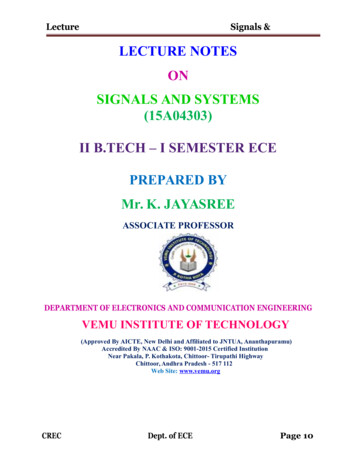
c J. Fessler, May 27, 2004, 13:11 (student version)4.15Can we implement h[n] with a finite number of adds, multiplies, delays? Only if H(z) is in rational form, which it is not! Itdoes not have an exact (finite) recursive implementation.How to make a practical implementation? A simple, but suboptimal approach: just truncate impulse response, since h[n] 0for large n. But how close will be the frequency response of this FIR approximation to ideal then? Let h[n], n NhN [n] 0,otherwise,and let HN (ω) be the corresponding frequency response:HN (ω) NXNXsin ωc n ωne.πnhN [n] e ωn n Nn NNo closed form for HN (ω). Use M ATLAB to compute HN (ω) and display.Truncated Sinc Filters0.5N0.510.3h10(n) H (ω) H(ω) N 100.40.20.40.30.50.100.20.10 0.1 0.2 80H (ω)N1.5 60 40 200204060800 505 505050ω51.50.50.5N 200.410.4h20(n)0.30.20.100.20.10 0.1 0.2 800.30.5 60 40 200204060800 505 51.50.50.5N 800.410.4h80(n)0.30.20.30.50.20.10 0.2 800.10 0.1 60 40 200n20406080 500ω5 5As N increases, hN [n] h[n]. But HN (ω) does not converge to H(ω) for every ω. But the energy difference of the two spectradecreases to 0 with increasing N . Practically, this is good enough.This effect, where truncating a sum in one domain leads to ringing in the other domain is called Gibbs phenomenon.We have just done our first filter design. It is a poor design though. Lots of taps, no recursive form, suboptimal approximation toideal lowpass for any given number of multiplies.

c J. Fessler, May 27, 2004, 13:11 (student version)4.164.2.5Energy density spectrum of aperiodic signals or Parseval’s relationE X X X Z π1 ωnx[n]x[n] x [n] x[n] X (ω) edω2π πn n n " #Z πZ πZ πX1112 ωnX (ω)x[n] eX (ω) X (ω) dω X (ω) dω .dω 2π π2π2π π πn 2 X1 x[n] 2πn 2Zπ π2 X (ω) dω .LHS: total energy of signal.RHS: integral of energy density over all frequencies.42Sxx (ω) X (ω) is called the energy density spectrum.When x[n] is aperiodic, the energy in any particular frequency is zero. ButZ ω212 X (ω) dω2π ω1quantifies how much energy the signal has in the frequency band [ω1 , ω2 ] for π ω1 ω2 πExample. x[n] an u[n] for a real. X(z) 11so X (ω) , so1 az 11 a e ω2Sxx (ω) X (ω) 11 a e ω2 1.1 2a cos ω a2Energy density spectrum of an u(n)a 0.54xxS (ω)32a 0.2a 0a 0.2a 0.510 50ω51a 0.5nx(n) a u(n)0.80.60.40.20 50n51010.5nx(n) a u(n)a 0.50 0.5 50n510Why is there greater energy density at high frequencies when a 0? Recall a n ( a )n ( 1)n a n which alternates.Note: for a 0 we have x[n] δ[n].

c J. Fessler, May 27, 2004, 13:11 (student version)

4.2 c J.Fessler,May27,2004,13:11(studentversion) Motivation: complex exponentials are eigenfunctions Why frequency analysis? Complex exponential signals, which are described by a frequency value, are eigenfunctions or eigensignals of LTI systems. Period signals, which are important in signal processing, are sums of complex exponential signals.