WIXLIB

Example:y(n) x(-n)y(n, t) T[x(n-t)] x(-n-t)y(n-t) x(-(n-t)) x(-n t) y(n, t) y(n-t). Hence, the system is time variant.Liner Time variant (LTV) and Liner Time Invariant (LTI) SystemsIf a system is both liner and time variant, then it is called liner time variant (LTV) system.If a system is both liner and time Invariant then that system is called liner time invariant (LTI)system.Static and Dynamic SystemsStatic system is memory-less whereas dynamic system is a memory system.Example 1: y(t) 2 x(t)For present value t 0, the system output is y(0) 2x(0). Here, the output is only dependent uponpresent input. Hence the system is memory less or static.Example 2: y(t) 2 x(t) 3 x(t-3)For present value t 0, the system output is y(0) 2x(0) 3x(-3).Here x(-3) is past value for the present input for which the system requires memory to get thisoutput. Hence, the system is a dynamic system.Causal and Non-Causal SystemsA system is said to be causal if its output depends upon present and past inputs, and does notdepend upon future input.For non causal system, the output depends upon future inputs also.Example 1: y(n) 2 x(t) 3 x(t-3)For present value t 1, the system output is y(1) 2x(1) 3x(-2).Here, the system output only depends upon present and past inputs. Hence, the system is causal.

Example 2: y(n) 2 x(t) 3 x(t-3) 6x(t 3)For present value t 1, the system output is y(1) 2x(1) 3x(-2) 6x(4) Here, the system outputdepends upon future input. Hence the system is non-causal system.Invertible and Non-Invertible systemsA system is said to invertible if the input of the system appears at the output.Y(S) X(S) H1(S) H2(S) X(S) H1(S) · 1(H1(S))Since H2(S) 1/( H1(S) ) Y(S) X(S) y(t) x(t)Hence, the system is invertible.If y(t) x(t), then the system is said to be non-invertible.Stable and Unstable SystemsThe system is said to be stable only when the output is bounded for bounded input. For abounded input, if the output is unbounded in the system then it is said to be unstable.Note: For a bounded signal, amplitude is finite.Example 1: y (t) x2(t)Let the input is u(t) (unit step bounded input) then the output y(t) u2(t) u(t) boundedoutput.Hence, the system is stable.

Example 2: y (t) x(t)dtLet the input is u (t) (unit step bounded input) then the output y(t) u(t)dt ramp signal(unbounded because amplitude of ramp is not finite it goes to infinite when t infinite).Hence, the system is unstable.Analogy Between Vectors and Signals:There is a perfect analogy between vectors and signals.VectorA vector contains magnitude and direction. The name of the vector is denoted by boldface type and their magnitude is denoted by light face type.Example: V is a vector with magnitude V. Consider two vectors V1 and V2 as shown in thefollowing diagram. Let the component of V1 along with V2 is given by C12V2. The component ofa vector V1 along with the vector V2 can obtained by taking a perpendicular from the end of V1to the vector V2 as shown in diagram:The vector V1 can be expressed in terms of vector V2V1 C12V2 VeWhere Ve is the error vector.But this is not the only way of expressing vector V1 in terms of V2. The alternate possibilitiesare:V1 C1V2 Ve1

V2 C2V2 Ve2The error signal is minimum for large component value. If C12 0, then two signals are said to beorthogonal.Dot Product of Two VectorsV1 . V2 V1.V2 cosθθ Angle between V1 and V2V1. V2 V2.V1From the diagram, components of V1 a long V2 C 12 V2

SignalThe concept of orthogonality can be applied to signals. Let us consider two signals f1(t) and f2(t).Similar to vectors, you can approximate f1(t) in terms of f2(t) asf1(t) C12 f2(t) fe(t) for (t1 t t2) fe(t) f1(t) – C12 f2(t)One possible way of minimizing the error is integrating over the interval t1 to t2.However, this step also does not reduce the error to appreciable extent. This can be corrected bytaking the square of error function.Where ε is the mean square value of error signal. The value of C12 which minimizes the error,you need to calculate dε/dC12 0Derivative of the terms which do not have C12 term are zero.Put C12 0 to get condition for orthogonality.

Orthogonal Vector SpaceA complete set of orthogonal vectors is referred to as orthogonal vector space. Consider a threedimensional vector space as shown below:Consider a vector A at a point (X1, Y1, Z1). Consider three unit vectors (VX, VY, VZ) in thedirection of X, Y, Z axis respectively. Since these unit vectors are mutually orthogonal, it satisfiesthatWe can write above conditions as

The vector A can be represented in terms of its components and unit vectors asAny vectors in this three dimensional space can be represented in terms of these three unitvectors only.If you consider n dimensional space, then any vector A in that space can be represented asAs the magnitude of unit vectors is unity for any vector AThe component of A along x axis A.VXThe component of A along Y axis A.VYThe component of A along Z axis A.VZSimilarly, for n dimensional space, the component of A along some G axis A.VG.(3)Substitute equation 2 in equation 3.

Orthogonal Signal SpaceLet us consider a set of n mutually orthogonal functions x 1(t), x2(t). xn(t) over theinterval t1 to t2. As these functions are orthogonal to each other, any two signals x j(t), xk(t) haveto satisfy the orthogonality condition. i.e.Let a function f(t), it can be approximated with this orthogonal signal space by adding thecomponents along mutually orthogonal signals i.e.The component which minimizes the mean square error can be found by

All terms that do not contain Ck is zero. i.e. in summation, r k term remains and all other termsare zero.Mean Square Error:The average of square of error function fe(t) is called as mean square error. It is denoted by ε(epsilon).

The above equation is used to evaluate the mean square error.Closed and Complete Set of Orthogonal Functions:Let us consider a set of n mutually orthogonal functions x1(t), x2(t).xn(t) over the intervalt1 to t2. This is called as closed and complete set when there exist no function f(t) satisfying theconditionIf this function is satisfying the equationFor k 1,2,. then f(t) is said to be orthogonal to each and every function of orthogonal set.This set is incomplete without f(t). It becomes closed and complete set when f(t) is included.f(t) can be approximated with this orthogonal set by adding the components along mutuallyorthogonal signals i.e.Orthogonality in Complex Functions:If f1(t) and f2(t) are two complex functions, then f1(t) can be expressed in terms of f2(t) asf1(t) C12f2(t). with negligible errorWhere f2*(t) is the complex conjugate of f2(t)If f1(t) and f2(t) are orthogonal then C12 0

The above equation represents orthogonality condition in complex functions.Fourier series:To represent any periodic signal x(t), Fourier developed an expression called Fourierseries. This is in terms of an infinite sum of sines and cosines or exponentials. Fourier series usesorthoganality condition.Jean Baptiste Joseph Fourier,a French mathematician and a physicist; was born inAuxerre, France. He initialized Fourier series, Fourier transforms and their applications toproblems of heat transfer and vibrations. The Fourier series, Fourier transforms and Fourier'sLaw are named in his honour.Fourier Series Representation of Continuous Time Periodic SignalsA signal is said to be periodic if it satisfies the condition x (t) x (t T) or x (n) x (n N).Where T fundamental time period,ω0 fundamental frequency 2π/TThere are two basic periodic signals:x(t) cosω0t(sinusoidal) &x(t) ejω0t(complex exponential)These two signals are periodic with period T 2π/ω0. A set of harmonically related complex exponentials can be represented as {ϕk(t)}All these signals are periodic with period T

According to orthogonal signal space approximation of a function x (t) with n, mutuallyorthogonal functions is given byWhere ak Fourier coefficient coefficient of approximation.This signal x(t) is also periodic with period T.Equation 2 represents Fourier series representation of periodic signal x(t).The term k 0 is constant.The term k 1 having fundamental frequency ω0 , is called as 1st harmonics.The term k 2 having fundamental frequency 2ω0 , is called as 2nd harmonics, and soon. The term k n having fundamental frequency nω0, is called as nth harmonics.Deriving Fourier CoefficientWe know thatMultiply e jnω0t on both sides. ThenConsider integral on both sides.

by Euler's formula,Hence in equation 2, the integral is zero for all values of k except at k n. Put k n inequation 2.Replace n by k

Properties of Fourier series:Linearity PropertyTime Shifting Property

Frequency Shifting PropertyTime Reversal PropertyTime Scaling PropertyDifferentiation and Integration Properties

Multiplication and Convolution PropertiesConjugate and Conjugate Symmetry Properties

Trigonometric Fourier Series (TFS)sinnω0t and sinmω0t are orthogonal over the interval (t0,t0 2πω0). So sinω0t,sin2ω0tforms an orthogonal set. This set is not complete without {cosnω0t } because this cosine set isalso orthogonal to sine set. So to complete this set we must include both cosine and sine terms.Now the complete orthogonal set contains all cosine and sine terms i.e. {sinnω0t,cosnω0t } wheren 0, 1, 2.The above equation represents trigonometric Fourier series representation of x(t).

Exponential Fourier Series (EFS):Consider a set of complex exponential functionswhich is orthogonal over the interval (t0,t0 T). Where T 2π/ω0 . This is a complete set so it ispossible to represent any function f(t) as shown belowEquation 1 represents exponential Fourier series representation of a signal f(t) over the interval(t0, t0 T). The Fourier coefficient is given as

Relation Between Trigonometric and Exponential Fourier Series:Consider a periodic signal x(t), the TFS & EFS representations are given below respectivelyCompare equation 1 and 2.Similarly,

Problems1. A continuous-time signal x ( t ) is shown in the following figure. Sketch and label eachof the following signals.( a ) x(t - 2); ( b ) x(2t);Sol:( c ) x(t/2);(d) x ( - t )

2. Determine whether the following signals are energy signals, power signals, orneither.(d) we know that energy of a signal isAnd by usingwe obtainThus, x [ n ] is a power signal.

(e) By the definition of power of signal3. Determine whether or not each of the following signals is periodic. If a signal isperiodic, determine its fundamental period.Sol:

1. Determine the even and odd components of the following signals:

UNIT – IICONTINUOUS TIMEFOURIER TRANSFORM

UNIT - IICONTINUOUS TIME FOURIER TRANSFORMINTRODUCTION:The main drawback of Fourier series is, it is only applicable to periodic signals. Thereare some naturally produced signals such as nonperiodic or aperiodic, which we cannotrepresent using Fourier series. To overcome this shortcoming, Fourier developed amathematical model to transform signals between time (or spatial) domain to frequency domain& vice versa, which is called 'Fourier transform'.Fourier transform has many applications in physics and engineering such as analysis ofLTI systems, RADAR, astronomy, signal processing etc.Deriving Fourier transform from Fourier series:Consider a periodic signal f(t) with period T. The complex Fourier series representationof f(t) is given as

In the limit as T ,Δf approaches differential df, kΔf becomes a continuous variable f, andsummation becomes integrationFourier transform of a signalInverse Fourier Transform is

Fourier Transform of Basic Functions:Let us go through Fourier Transform of basic functions:FT of GATE FunctionFT of Impulse Function:FT of Unit Step Function:FT of Exponentials:

FT of Signum Function :Conditions for Existence of Fourier Transform:Any function f(t) can be represented by using Fourier transform only when the functionsatisfies Dirichlet’s conditions. i.e. The function f(t) has finite number of maxima and minima. There must be finite number of discontinuities in the signal f(t),in the given interval oftime. It must be absolutely integrable in the given interval of time i.e.Properties of Fourier Transform:Here are the properties of Fourier Transform:Linearity Property:Then linearity property states that

Time Shifting Property:Then Time shifting property states thatFrequency Shifting Property:Then frequency shifting property states thatTime Reversal Property:Then Time reversal property states thatTime Scaling Property:Then Time scaling property states thatDifferentiation and Integration Properties:

Then Differentiation property states thatand integration property states thatMultiplication and Convolution Properties:Then multiplication property states thatand convolution property states thatSampling Theorem and its Importance:

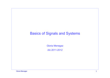
Statement of Sampling Theorem:A band limited signal can be reconstructed exactly if it is sampled at a rate atleast twicethe maximum frequency component in it."The following figure shows a signal g(t) that is bandlimited.Figure1: Spectrum of band limited signal g(t)The maximum frequency component of g(t) is fm. To recover the signal g(t) exactly from itssamples it has to be sampled at a rate fs 2fm.The minimum required sampling rate fs 2fm is called “Nyquist rate”.Proof:Let g(t) be a bandlimited signal whose bandwidth is fm (ωm 2πfm).Figure 2: (a) Original signal g(t) (b) Spectrum G(ω)

Figure 3:Let gs(t) be the sampled signal. Its Fourier Transform Gs(ω) is given by

Aliasing:Aliasing is a phenomenon where the high frequency components of the sampled signalinterfere with each other because of inadequate sampling ωs ωmAliasing leads to distortion in recovered signal. This is the reason why samplingfrequency should be atleast twice the bandwidth of the signal.

Oversampling:In practice signal are oversampled, where fs is signi cantly higher than Nyquist rate toavoid aliasing.Problems1. Find the Fourier transform of the rectangular pulse signal x(t) defined bySol: By definition of Fourier transform

Hence we obtainThe following figure shows the Fourier transform of the given signal x(t)Figure: Fourier transform of the given signal2. Find the Fourier transform of the following signal x(t)Sol: Signal x(t) can be rewritten as

Hence, we getThe Fourier transform X(w) of x(t) is shown in the following figures(a)(b)Fig: (a) Signal x(t) (b) Fourier transform X(w) of x(t)4. Find the Fourier transform of the periodic impulse trainFig: Train of impulsesSol: Given signal can be written as

Thus, the Fourier transform of a unit impulse train is also a similar impulse train. The followingfigure shows the Fourier transform of a unit impulse trainFigure: Fourier transform of the given signal5.Find the Fourier transform of the signum functionSol: Signum function is defined asThe signum function, sgn(t), can be expressed asSgn(t) 2u(t)-1

We know thatFig: Signum functionLetThen applying the differentiation property , we haveNote that sgn(t) is an odd function, and therefore its Fourier transform is a pure imaginaryfunction of w

Properties of Fourier Transform:

Fourier Transform of Basic Functions:

DISCRETE TIME FOURIER TRANSFORMDiscrete Time Fourier Transforms (DTFT)Here we take the exponential signals to bewhere is a real number.Therepresentation is motivated by the Harmonic analysis, but instead of following the historicaldevelopment of the representation wegive directly the defining equation.Letbe discrete time signal such thatthat is sequence is absolutelysummable.The sequencecan be represented by a Fourier integral of the form.(1)Where(2)Equation (1) and (2) give the Fourier representation of the signal. Equation (1) is referredas synthesis equation or the inverse discrete time Fourier transform (IDTFT) and equation (2)isFourier transform in the analysis equation. Fourier transform of a signal in general is a complexvalued function, we can writewhereis magnitude andis the phase of. We also use the term Fourierspectrum or simply, the spectrum to refer to. Thusis called the magnitude spectrum andis called the phase spectrum. From equation (2) we can see thatis a periodicfunction with periodi.e. We can interpret (1) as Fourier coefficients in the representation ofa periodic function. In the Fourier series analysis our attention is on the periodic function, herewe are concerned with the representation of the signal. So the roles of the two equation areinterchanged compared to the Fourier series analysis of periodic signals.Now we show that if we put equation (2) in equation (1) we indeed get the signal.Letwhere we have substitutedfrom (2) into equation (1) and called the result as.Since we have used n as index on the left hand side we have used m as the index variable for the

sum defining the Fourier transform. Under our assumption thatsequence is absolutelysummable we can interchange the order of integration and summation. ThusExample: LetFourier transform of this sequence will exist if it is absolutely summable. We have

Fourier transform of Periodic SignalsFor a periodic discrete-time signal,its Fourier transform of this signal is periodic in w with period 2 , and is givenNow consider a periodic sequence x[n] with period N and with the Fourier series representationThe Fourier transform is

Properties of the Discrete Time Fourier Transform:Letandbe two signal, then their DTFT is denoted byis used to say that left hand side is the signal x[n] whose DTFT isside.1. Periodicity of the DTFT:2. Linearity of the DTFT:3. Time Shifting and Frequency Shifting:and. The notationis given at right hand

4. Conjugation and Conjugate Symmetry:From this, it follows that Re X(e jw ) is an even function of w and Im X (e jw ) is an odd function of w . Similarly, the magnitude of X(e jw ) is an even function and thephase angle isan odd function. Furthermore,5. Differencing and Accumulation

The impulse train on the right-hand side reflects the dc or average value that can result fromsummation.For example, the Fourier transform of the unit step x[n] u[n] can be obtained by usingthe accumulation property.6. Time Reversal7. Time ExpansionFor

UNIT III:SIGNAL TRANSMISSION THROUGH LINEAR SYSTEMS: Linear system, impulse response, Response of a linear system, linear time-invariant (LTI) system, linear time variant (LTV) system, Transfer function of a LTI system. Filter . "Signals & Systems", Wiley, 2nd Edition. 2. B.P. Lathi, "Signals, Systems & Communications", 2009,BS .