WIXLIB

922. Satisfiability Solversits subformulas. For instance, given an arbitrary propositional formula G, one wouldfirst locally re-write each of its logic operators in terms of , , and to obtain, say,G (((a b) ( a b)) c) d. To convert this to CNF, one possibility is to addfour auxiliary variables w, x, y, and z, construct clauses that encode the four relationsw (a b), x ( a b), y (w x), and z (y c), and add to that the clause(z d).2.2SAT Solver Technology—Complete MethodsA complete solution method for the SAT problem is one that, given the input formulaF, either produces a satisfying assignment for F or proves that F is unsatisfiable.One of the most surprising aspects of the relatively recent practical progress of SATsolvers is that the best complete methods remain variants of a process introducedseveral decades ago: the DPLL procedure, which performs a backtrack search in thespace of partial truth assignments. A key feature of DPLL is efficient pruning of thesearch space based on falsified clauses. Since its introduction in the early 1960’s, themain improvements to DPLL have been smart branch selection heuristics, extensionslike clause learning and randomized restarts, and well-crafted data structures such aslazy implementations and watched literals for fast unit propagation. This section isdevoted to understanding these complete SAT solvers, also known as “systematic”solvers.32.2.1The DPLL ProcedureThe Davis-Putnam-Logemann-Loveland or DPLL procedure is a complete, systematic search process for finding a satisfying assignment for a given Boolean formula orproving that it is unsatisfiable. Davis and Putnam [61] came up with the basic ideabehind this procedure. However, it was only a couple of years later that Davis, Logemann, and Loveland [60] presented it in the efficient top-down form in which it iswidely used today. It is essentially a branching procedure that prunes the search spacebased on falsified clauses.Algorithm 1, DPLL-recursive(F, ρ ), sketches the basic DPLL procedure onCNF formulas. The idea is to repeatedly select an unassigned literal in the inputformula F and recursively search for a satisfying assignment for F and F . Thestep where such an is chosen is commonly referred to as the branching step. Setting to TRUE or FALSE when making a recursive call is called a decision, and is associated with a decision level which equals the recursion depth at that stage. The endof each recursive call, which takes F back to fewer assigned variables, is called thebacktracking step.A partial assignment ρ is maintained during the search and output if the formulaturns out to be satisfiable. If F ρ contains the empty clause, the corresponding clauseof F from which it came is said to be violated by ρ . To increase efficiency, unit clausesare immediately set to TRUE as outlined in Algorithm 1; this process is termed unit3 Due to space limitation, we cannot do justice to a large amount of recent work on complete SATsolvers, which consists of hundreds of publications. The aim of this section is to give the reader an overviewof several techniques commonly employed by these solvers.

C.P. Gomes et al.93Algorithm 2.1: DPLL-recursive(F, ρ )Input : A CNF formula F and an initially empty partial assignment ρOutput : UNSAT, or an assignment satisfying Fbegin(F, ρ ) UnitPropagate(F, ρ )if F contains the empty clause then return UNSATif F has no clauses left thenOutput ρreturn SAT a literal not assigned by ρ// the branching stepif DPLL-recursive(F , ρ { }) SAT then return SATreturn DPLL-recursive(F , ρ { })endsub UnitPropagate(F, ρ )beginwhile F contains no empty clause but has a unit clause x doF F xρ ρ {x}return (F, ρ )endpropagation. Pure literals (those whose negation does not appear) are also set toTRUE as a preprocessing step and, in some implementations, during the simplificationprocess after every branch.Variants of this algorithm form the most widely used family of complete algorithms for formula satisfiability. They are frequently implemented in an iterativerather than recursive manner, resulting in significantly reduced memory usage. Thekey difference in the iterative version is the extra step of unassigning variables whenone backtracks. The naive way of unassigning variables in a CNF formula is computationally expensive, requiring one to examine every clause in which the unassignedvariable appears. However, the watched literals scheme provides an excellent wayaround this and will be described shortly.2.2.2Key Features of Modern DPLL-Based SAT SolversThe efficiency of state-of-the-art SAT solvers relies heavily on various features thathave been developed, analyzed, and tested over the last decade. These include fastunit propagation using watched literals, learning mechanisms, deterministic and randomized restart strategies, effective constraint database management (clause deletionmechanisms), and smart static and dynamic branching heuristics. We give a flavor ofsome of these next.Variable (and value) selection heuristic is one of the features that vary the mostfrom one SAT solver to another. Also referred to as the decision strategy, it can havea significant impact on the efficiency of the solver (see e.g. [160] for a survey). Thecommonly employed strategies vary from randomly fixing literals to maximizing amoderately complex function of the current variable- and clause-state, such as the

942. Satisfiability SolversMOMS (Maximum Occurrence in clauses of Minimum Size) heuristic [121] or theBOHM heuristic [cf. 32]. One could select and fix the literal occurring most frequently in the yet unsatisfied clauses (the DLIS (Dynamic Largest Individual Sum)heuristic [161]), or choose a literal based on its weight which periodically decays butis boosted if a clause in which it appears is used in deriving a conflict, like in theVSIDS (Variable State Independent Decaying Sum) heuristic [170]. Newer solverslike BerkMin [93], Jerusat [171], MiniSat [71], and RSat [184] employ furthervariations on this theme.Clause learning has played a critical role in the success of modern completeSAT solvers. The idea here is to cache “causes of conflict” in a succinct manner (aslearned clauses) and utilize this information to prune the search in a different part ofthe search space encountered later. We leave the details to Section 2.2.3, which willbe devoted entirely to clause learning. We will also see how clause learning provablyexponentially improves upon the basic DPLL procedure.The watched literals scheme of Moskewicz et al. [170], introduced in their solverzChaff, is now a standard method used by most SAT solvers for efficient constraintpropagation. This technique falls in the category of lazy data structures introducedearlier by Zhang [236] in the solver Sato. The key idea behind the watched literalsscheme, as the name suggests, is to maintain and “watch” two special literals foreach active (i.e., not yet satisfied) clause that are not FALSE under the current partialassignment; these literals could either be set to TRUE or be as yet unassigned. Recallthat empty clauses halt the DPLL process and unit clauses are immediately satisfied.Hence, one can always find such watched literals in all active clauses. Further, aslong as a clause has two such literals, it cannot be involved in unit propagation. Theseliterals are maintained as follows. Suppose a literal is set to FALSE. We performtwo maintenance operations. First, for every clause C that had as a watched literal,we examine C and find, if possible, another literal to watch (one which is TRUE orstill unassigned). Second, for every previously active clause C 0 that has now becomesatisfied because of this assignment of to FALSE, we make a watched literal forC0 . By performing this second step, positive literals are given priority over unassignedliterals for being the watched literals.With this setup, one can test a clause for satisfiability by simply checking whetherat least one of its two watched literals is TRUE. Moreover, the relatively small amountof extra book-keeping involved in maintaining watched literals is well paid off whenone unassigns a literal by backtracking—in fact, one needs to do absolutely nothing!The invariant about watched literals is maintained as such, saving a substantial amountof computation that would have been done otherwise. This technique has played acritical role in the success of SAT solvers, in particular those involving clause learning. Even when large numbers of very long learned clauses are constantly added tothe clause database, this technique allows propagation to be very efficient—the longadded clauses are not even looked at unless one assigns a value to one of the literalsbeing watched and potentially causes unit propagation.Conflict-directed backjumping, introduced by Stallman and Sussman [220], allows a solver to backtrack directly to a decision level d if variables at levels d or lowerare the only ones involved in the conflicts in both branches at a point other than thebranch variable itself. In this case, it is safe to assume that there is no solution extending the current branch at decision level d, and one may flip the corresponding variable

C.P. Gomes et al.95at level d or backtrack further as appropriate. This process maintains the completenessof the procedure while significantly enhancing the efficiency in practice.Fast backjumping is a slightly different technique, relevant mostly to the nowpopular FirstUIP learning scheme used in SAT solvers Grasp [161] and zChaff [170].It lets a solver jump directly to a lower decision level d when even one branch leadsto a conflict involving variables at levels d or lower only (in addition to the variableat the current branch). Of course, for completeness, the current branch at level d isnot marked as unsatisfiable; one simply selects a new variable and value for leveld and continues with a new conflict clause added to the database and potentially anew implied variable. This is experimentally observed to increase efficiency in manybenchmark problems. Note, however, that while conflict-directed backjumping is always beneficial, fast backjumping may not be so. It discards intermediate decisionswhich may actually be relevant and in the worst case will be made again unchangedafter fast backjumping.Assignment stack shrinking based on conflict clauses is a relatively new technique introduced by Nadel [171] in the solver Jerusat, and is now used in othersolvers as well. When a conflict occurs because a clause C 0 is violated and the resulting conflict clause C to be learned exceeds a certain threshold length, the solverbacktracks to almost the highest decision level of the literals in C. It then starts assigning to FALSE the unassigned literals of the violated clause C 0 until a new conflictis encountered, which is expected to result in a smaller and more pertinent conflictclause to be learned.Conflict clause minimization was introduced by Eén and Sörensson [71] in theirsolver MiniSat. The idea is to try to reduce the size of a learned conflict clauseC by repeatedly identifying and removing any literals of C that are implied to beFALSE when the rest of the literals in C are set to FALSE . This is achieved usingthe subsumption resolution rule, which lets one derive a clause A from (x A) and( x B) where B A (the derived clause A subsumes the antecedent (x A)). Thisrule can be generalized, at the expense of extra computational cost that usually paysoff, to a sequence of subsumption resolution derivations such that the final derivedclause subsumes the first antecedent clause.Randomized restarts, introduced by Gomes et al. [102], allow clause learningalgorithms to arbitrarily stop the search and restart their branching process from decision level zero. All clauses learned so far are retained and now treated as additionalinitial clauses. Most of the current SAT solvers, starting with zChaff [170], employaggressive restart strategies, sometimes restarting after as few as 20 to 50 backtracks.This has been shown to help immensely in reducing the solution time. Theoretically,unlimited restarts, performed at the correct step, can provably make clause learningvery powerful. We will discuss randomized restarts in more detail later in the chapter.2.2.3Clause Learning and Iterative DPLLAlgorithm 2.2 gives the top-level structure of a DPLL-based SAT solver employingclause learning. Note that this algorithm is presented here in the iterative format(rather than recursive) in which it is most widely used in today’s SAT solvers.The procedure DecideNextBranch chooses the next variable to branch on (andthe truth value to set it to) using either a static or a dynamic variable selection heuris-

2. Satisfiability Solvers96Algorithm 2.2: DPLL-ClauseLearning-IterativeInput : A CNF formulaOutput : UNSAT, or SAT along with a satisfying assignmentbeginwhile TRUE doDecideNextBranchwhile TRUE dostatus Deduceif status CONFLICT thenblevel AnalyzeConflictif blevel 0 then return UNSATBacktrack(blevel)else if status SAT thenOutput current assignment stackreturn SATelse breakendtic. The procedure Deduce applies unit propagation, keeping track of any clauses thatmay become empty, causing what is known as a conflict. If all clauses have been satisfied, it declares the formula to be satisfiable.4 The procedure AnalyzeConflictlooks at the structure of implications and computes from it a “conflict clause” to learn.It also computes and returns the decision level that one needs to backtrack. Note thatthere is no explicit variable flip in the entire algorithm; one simply learns a conflictclause before backtracking, and this conflict clause often implicitly “flips” the valueof a decision or implied variable by unit propagation. This will become clearer whenwe discuss the details of conflict clause learning and unique implication point.In terms of notation, variables assigned values through the actual variable selection process (DecideNextBranch) are called decision variables and those assignedvalues as a result of unit propagation (Deduce) are called implied variables. Decisionand implied literals are analogously defined. Upon backtracking, the last decisionvariable no longer remains a decision variable and might instead become an impliedvariable depending on the clauses learned so far. The decision level of a decisionvariable x is one more than the number of current decision variables at the time ofbranching on x. The decision level of an implied variable y is the maximum of thedecision levels of decision variables used to imply y; if y is implied a value withoutusing any decision variable at all, y has decision level zero. The decision level at anystep of the underlying DPLL procedure is the maximum of the decision levels of allcurrent decision variables, and zero if there is no decision variable yet. Thus, for instance, if the clause learning algorithm starts off by branching on x, the decision levelof x is 1 and the algorithm at this stage is at decision level 1.A clause learning algorithm stops and declares the given formula to be unsatisfiable whenever unit propagation leads to a conflict at decision level zero, i.e., when4 In some implementations involving lazy data structures, solvers do not keep track of the actualnumber of satisfied clauses. Instead, the formula is declared to be satisfiable when all variables have beenassigned truth values and no conflict is created by this assignment.

C.P. Gomes et al.97no variable is currently branched upon. This condition is sometimes referred to as aconflict at decision level zero.Clause learning grew out of work in artificial intelligence seeking to improve theperformance of backtrack search algorithms by generating explanations for failure(backtrack) points, and then adding the explanations as new constraints on the originalproblem. The results of Davis [62], de Kleer and Williams [63], Dechter [64], Genesereth [82], Stallman and Sussman [220], and others proved this approach to be quitepromising. For general constraint satisfaction problems the explanations are called“conflicts” or “no-goods”; in the case of Boolean CNF satisfiability, the techniquebecomes clause learning—the reason for failure is learned in the form of a “conflictclause” which is added to the set of given clauses. Despite the initial success, the earlywork in this area was limited by the large numbers of no-goods generated during thesearch, which generally involved many variables and tended to slow the constraintsolvers down. Clause learning owes a lot of its practical success to subsequent research exploiting efficient lazy data structures and constraint database managementstrategies. Through a series of papers and often accompanying solvers, BayardoJr. and Miranker [17], Bayardo Jr. and Schrag [19], Marques-Silva and Sakallah[161], Moskewicz et al. [170], Zhang [236], Zhang et al. [240], and others showedthat clause learning can be efficiently implemented and used to solve hard problemsthat cannot be approached by any other technique.In general, the learning process hidden in AnalyzeConflict is expected to saveus from redoing the same computation when we later have an assignment that causesconflict due in part to the same reason. Variations of such conflict-driven learninginclude different ways of choosing the clause to learn (different learning schemes)and possibly allowing multiple clauses to be learned from a single conflict. We nextformalize the graph-based framework used to define and compute conflict clauses.Implication Graph and ConflictsUnit propagation can be naturally associated with an implication graph that capturesall possible ways of deriving all implied literals from decision literals. In what follows, we use the term known clauses to refer to the clauses of the input formula aswell as to all clauses that have been learned by the clause learning process so far.Definition 1. The implication graph G at a given stage of DPLL is a directed acyclicgraph with edges labeled with sets of clauses. It is constructed as follows:Step 1: Create a node for each decision literal, labeled with that literal. Thesewill be the indegree-zero source nodes of G.Step 2: While there exists a known clause C (l1 . . . lk l) such that l1 , . . . , lklabel nodes in G,i. Add a node labeled l if not already present in G.ii. Add edges (li , l), 1 i k, if not already present.iii. Add C to the label set of these edges. These edges are thought of asgrouped together and associated with clause C.

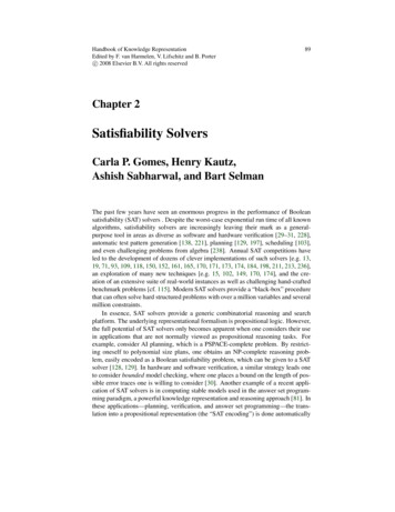
2. Satisfiability Solvers98Step 3: Add to G a special “conflict” node Λ. For any variable x that occurs bothpositively and negatively in G, add directed edges from x and x to Λ.Since all node labels in G are distinct, we identify nodes with the literals labelingthem. Any variable x occurring both positively and negatively in G is a conflict variable , and x as well as x are conflict literals. G contains a conflict if it has at leastone conflict variable. DPLL at a given stage has a conflict if the implication graph atthat stage contains a conflict. A conflict can equivalently be thought of as occurringwhen the residual formula contains the empty clause Λ. Note that we are using Λ todenote the node of the implication graph representing a conflict, and Λ to denote theempty clause.By definition, the implication graph may not contain a conflict at all, or it maycontain many conflict variables and several ways of deriving any single literal. Tobetter understand and analyze a conflict when it occurs, we work with a subgraph ofthe implication graph, called the conflict graph (see Figure 2.1), that captures only oneamong possibly many ways of reaching a conflict from the decision variables usingunit propagation.a cut correspondingto clause ( a b)conflictvariable py x1a q tΛ x2 yb x3reason sideconflict sideFigure 2.1: A conflict graphDefinition 2. A conflict graph H is any subgraph of the implication graph with thefollowing properties:(a) H contains Λ and exactly one conflict variable.

example, consider AI planning, which is a PSPACE-complete problem. By restrict-ing oneself to polynomial size plans, one obtains an NP-complete reasoning prob-lem, easily encoded as a Boolean satisability problem, which can be given to a SAT solver [128, 129]. In hardware and software verication, a similar strategy leads one