Transcription
New Features of PopulationSynthesis:PopSyn III of CT-RAMPPeter Vovsha, Jim Hicks, Binny Paul, PBVladimir Livshits, Kyunghwi Jeon, PetyaManeva, MAGITM, Baltimore, MD, April 27-30, 20141
1. MOTIVATION & STATEMENTOF INNOVATIONSITM, Baltimore, MD, April 27-30, 20142
Previous Generation of PopulationSynthesizers Problem formulation: 3 Steps: Create a list of HHs in each TAZ from a sample (PUMS)Match the given controls(“Balance”) Multidimensional HH distribution in each TAZ(“Dicretize”) List of HHs with controlled variables in each TAZ(“Draw”) Randomly join HHs from PUMS by controlledvariablesLimitations: No single theoretical framework / no guarantee of uniquesolution / no method to compare different solutionsDifficult to handle both HH and person characteristicsEach HH characteristic has to be presented as a distribution;no convenient way to introduce general tendenciesITM, Baltimore, MD, April 27-30, 20143
State of the Art Analytical methods that balance a “list” (orsample) of HHs to meet the controlsimposed at some level of geography (TAZ)[Bar-Gera et al all, 2012, Ye et al, 2009]: PopSyn III belongs to this familyCombinatorial methods based on arandom swapping on HHs between TAZs ifthe fit measures can be improved[Abraham et al, 2012; Harland et al, 2012]ITM, Baltimore, MD, April 27-30, 20144
Our Contribution General formulation of convergence of the balancing procedurewith imperfect (i.e. not fully consistent) controls: Optimized discretizing of the fractional outcomes of the balancingprocedure to form a list of discrete households: Guarantees unique repeatable solutionScreens inconsistencies and addresses a differential degree ofconfidence in different controlsEnhanced spatial resolution and growing number of controls makerounding errors substantial w/simple “bucket” roundingLinear Programming (LP) approach in order to optimize the discretizedweights and preserve the best possible match to the controlsEliminates Monte-Carlo simulation error, all procedures are analyticaland repeatableMultiple levels of geography where the controls can be set: Important demographic and socio-economic trends can only betranslated into more aggregate controls than a TAZ-level controlIn new generation of ABMs all location choices are modeled at thelevel of Micro-Analysis Zones (MAZs) nested within TAZsITM, Baltimore, MD, April 27-30, 20145
2. CORE LIST BALANCINGITM, Baltimore, MD, April 27-30, 20146
List of Individual HHsHH ID1i 1n 1n 2n 3n 4n 5 .ControlHH size23i 2i 34 i 40-15i 5Person age16-35 36-64i 6i 71i 81111111123300400400110065 200250ITM, Baltimore, MD, April 27-30, 2014222650HHinitialweight n2020202020 2507
Basic Formulation of ListBalancing w/Fixed Controls- Preserve initial weights as much as possible- Meet all controls Convex mathematical program with linear constraintsSolution can be found by forming the Lagrangian and equatingpartial derivatives to zero (necessary conditions)Conventional matrix balancing or table balancing are particularcasesITM, Baltimore, MD, April 27-30, 20148
Solution Does not guarantee existence of the solution(feasibility of constraints)Scale k is incorporated in balancing factors only ifthe total weight (number of HHs) is predefined bycontrolsIf constraints are feasible and total weight (numberof HHs) is predefined, a solution exists, it is unique,and independent of the scale of initial weightsCan be found by Newton-Raphson but a simplebalancing method also works wellITM, Baltimore, MD, April 27-30, 20149
Relaxation of Controls Objective function: Match relaxed controls: HH weights and relaxation factors: Importance factors for controls: Large value of 1,000 to ensure match if feasible1,000,000 for total number of HHsITM, Baltimore, MD, April 27-30, 201410
Solution w/Relaxation Guarantees existence of the solution (regardlessof feasibility of constraints)If constraints are feasible and importance factorsare large the solution is equivalent to solution ofthe problem w/o relaxationNewton-Raphson method to calculate balancingfactors efficiently Relaxation of constraints included in the loop withadjustment of weightsITM, Baltimore, MD, April 27-30, 201411
Iterative Application of NewtonRaphson MethodFor each iterationFor each control//Step 1: Calculate balancing factors// Step 2: Update HH weights:// Step 3: Update relaxation factors:End of loop over controls// Step 4: Check for convergenceEnd of loop over iterationsITM, Baltimore, MD, April 27-30, 201412
How Relaxation Works If the controls are consistent: Algorithm performs exactly as balancing algorithmw/fixed constraints and yields the same solutionIf the controls are internally inconsistent: Balancing w/o relaxations does not converge at allBalancing w/relaxations produces a uniqueconvergent solution w/controls satisfied to theextent possibleDegree of the necessary relaxation of each controlis inversely related to the importance weightITM, Baltimore, MD, April 27-30, 201413
3. DISCRETIZINGITM, Baltimore, MD, April 27-30, 201414
Discretizing is Not Trivial Discretizing is not a trivial problem: Simple rounding may cause substantial deviations fromthe controls: Population is synthesized at a fine level of spatial resolution(30,000-40,000 MAZs)Balancing results in many small fractional numbersAccumulated across multiple MAZsIf rounding is forced to match controls exactly it may causesignificant deviation from the distribution of initial weightsDiscretizing problem can be formulated as replacing thefractional household weights with integer weights that: Preserves controls as well as possible andAchieve uniformity of HH weights to the maximum extentITM, Baltimore, MD, April 27-30, 201415
Discretizing as LP Problem Objective function – discrete weights asclose as possible to original fractionalweights: yn ln , ifmin yn xn nif 0 yn 1 max yn ln xn nyn 0 S.T. constraints – matching residualcontrols: anni yn Aiyn 0,1ITM, Baltimore, MD, April 27-30, 201416
4. MULTIPLE LEVEL OFGEOGRAPHYITM, Baltimore, MD, April 27-30, 201417
Multiple Levels of GeographyNeeded for Setting Controls Important demographic & socio-economictrends: Can only be translated into more aggregatecontrols than TAZ-levelHandled by upward meta-balancingNew generation of CT-RAMP ABMs operate withenhanced level of spatial resolution: Location choices are modeled at the level ofMicro-Analysis Zones (MAZs) nested within TAZsHandled by downward allocationITM, Baltimore, MD, April 27-30, 201418
Workers-Jobs Balance Generated workers by industry shouldcorrespond to job segmentation byindustry: Regional levelDiscrepancies eliminated: (Standard way) regional normalization of#jobs by industry to match #workers(Suggested way) adding workers-by-industrymeta-control to PopSynITM, Baltimore, MD, April 27-30, 201419
5. UPWARD METABALANCINGITM, Baltimore, MD, April 27-30, 201420
Decomposition for MetaBalancing Meta-controls can be written rigorously asextension of the core List Balancingprocedure: HH weights optimized simultaneously for allTAZs in the region accounting for controls atTAZ level as well as upper levels of geographyUseful for theoretical analysis but impracticaldue to huge dimensionalityThus, the problem has to be decomposedITM, Baltimore, MD, April 27-30, 201421
HH distributions by size,income, #workers for each TAZBalance individual HHs in eachTAZWorkers by industry foreach TAZWorker distribution by industryfor each countyBalance workers by industryfor each TAZ in countyITM, Baltimore, MD, April 27-30, 2014Worker distribution byindustry for each TAZMeta-Balancing22
5. DOWNWARD ALLOCATIONFROM PUMA TO TAZ & FROMTAZ TO MAZITM, Baltimore, MD, April 27-30, 201423
Allocation Procedure Allocate HH weights generated from any upperlevel of geography to the lower level of geography: PUMA to TAZsTAZ to MAZsBalancing-and-discretizing procedure appliedsequentially to each MAZ in the TAZ: MAZs from smallest to biggest in terms of #HHsTAZ-level HH weights as initial weightsResidual weights are adjusted w/o replacementTotal weight summed across the MAZs is matched tothe original TAZ-level weight for each HHITM, Baltimore, MD, April 27-30, 201424
Balancing & Discretizing (PUMA-Meta)Controls by geographySample of HHsList balancingMeta balancingHHs from PUMAw/replacementPUMA:· HH size (1,2,3,4 )· HH income (5 quintiles)· Housing type (1,2)· #university studentsHHs balanced for PUMA withfractional weights# workers byindustry for eachPUMABalanced # workersby industry for eachPUMACounty (MAG, PAG):· Workers by industryHHs balanced for PUMA withfractional weightsHHs discretized for PUMAwith weights 1HHs discretized for PUMAwith residual weights 1 by LPITM, Baltimore, MD, April 27-30, 201425
Balancing & Discretizing (PUMA-TAZ)HHs from PUMAw/o replacementTAZ:· HH size (1,2,3,4 )· HH income (5 quintiles)· Housing type (1,2)· #university studentsHHs balanced for TAZ withfractional weightsHHs discretized for TAZ withweights 1HHs discretized for TAZ withresidual weights 1 by LPTAZs within PUMA are processed from smallest to biggestITM, Baltimore, MD, April 27-30, 201426
Balancing & Discretizing (TAZ-MAZ)HHs from TAZ w/oreplacementMAZ:· HH size (1,2,3,4 )· HH income (5 quintiles)· #university studentsHHs balanced for MAZ withfractional weightsHHs discretized for MAZ withweights 1HHs discretized for MAZ withresidual weights 1 by LPMAZs within TAZ are processed from smallest to biggestITM, Baltimore, MD, April 27-30, 201427
PopSyn III:MAG Input Highlights Region: MAG (4 Counties)No of PUMAs in Modeling region: 24No of TAZs: 3,009No of MAZs: 26,231Seed Sample: PUMS (ACS 2006-10, 5% sample)Max Expansion Factor: 5Controls: Total no of HHs, very high importance, MAZHH size categories (1,2,3,4 ), med imp, MAZIncome quintiles, med imp, MAZHousing type (single/multi-family), med imp, MAZPerson age categories (0-18,19-35,36-65,66 ), med imp,MAZ#Workers by industry type, med imp, META (district)ITM, Baltimore, MD, April 27-30, 201428
Uniformity of HH ExpansionFactors Ensured by initial balancing of HHweights at PUMA level: Subsequent allocation to TAZ and MAZ w/oreplacement preserves expansionCannot be achieved by independentbalancing of HH weights for each MAZ: Results in very “lumpy” weightsITM, Baltimore, MD, April 27-30, 201429
6. POPSYN VALIDATIONITM, Baltimore, MD, April 27-30, 201430
Dimensions for PopSyn Validation PopSyn Input: Controls vs. Sample (PUMA): Substantial discrepancies can start here andnot necessarily wrongPopSyn Output: Matching controls (MAZ, TAZ, PUMA, Meta)Uniformity of HH expansion factors (PUMA)Uncontrolled variables vs. PUMA/CensusITM, Baltimore, MD, April 27-30, 201431
7. CONSISTENCY OF POPSYNINPUTITM, Baltimore, MD, April 27-30, 201432
Control vs. PUMSPUMA 103HH Size0.35Percentage0.30.25PUMA (weighted)0.2Controls0.150.10.050ITM, Baltimore, MD, April 27-30, 201433
PercentMeta-Controls vs. PUMSMAG Region0.140.120.10.080.060.040.020MAG RegionPUMS SampleControlsIndustryITM, Baltimore, MD, April 27-30, 201434
Reasons for Discrepancy Different years: Sampling error: PUMS is multi-year sampleControls set for a single base yearPUMS is 5% sampleControls reflect independent sources and/or LUmodel forecasts for the entire populationImplications: From the very beginning we cannot expect a fullmatch, moreover we may intentionally skewsynthetic populationITM, Baltimore, MD, April 27-30, 201435
8. MATCHING CONTROLSITM, Baltimore, MD, April 27-30, 201436
Matching Controls at RegionalLevelVariablePopulationTotal HHHHsize1HHsize2HHsize3HHsize4 ge3665Age66 Single FamilyMulti ,516,213437,0571,278,227261,921ITM, Baltimore, MD, April 27-30, .030%-0.021%-0.003%0.016%37
Meta-Controls at Regional LevelNAICS ing I8,775Manufacturing II26,010Manufacturing III89,961Wholesale83,227Retail I140,999Retail II74,694Transportation35,508Transportation - Postal15,382Information30,599Finance I95,247Finance II49,209Professional I152,171Professional II4,085Professional itary220,967ITM, Baltimore, MD, April 27-30, 13%0.049%-0.055%38
PUMA Level Matching – Example(PUMA 101)VariableTotal HHHHsize1HHsize2HHsize3HHsize4 ge3665Age66 Single FamilyMulti 549ITM, Baltimore, MD, April 27-30, 039%-0.003%0.056%39
TAZ Level Matching – Example(TAZ 108)VariableTotal HHHHsize1HHsize2HHsize3HHsize4 ge3665Age66 Single FamilyMulti 92253173487ITM, Baltimore, MD, April 27-30, .000%0.000%40
TAZ Level Matching – Example(TAZ 2191)VariableTotal HHHHsize1HHsize2HHsize3HHsize4 ge3665Age66 Single FamilyMulti , Baltimore, MD, April 27-30, 0.883%0.043%-0.791%41
Why Cannot Controls be Matchedfor TAZ 2191? The reason is always a structuralinconsistency between the controlsthemselves as well as between thecontrols and sample proportions: Controls want a few large HHs and a fewchildrenControls want more retired HHsControls want more high-income HHs at thesame timeThese controls cannot be fully reconciled andPopSyn finds the best compromise solutionITM, Baltimore, MD, April 27-30, 201442
TAZ Level MatchingScatter Plot : [Output-Control]Total # HHs ControlFrequency - (Control - 0100200300Difference between TAZ Control and Model OutputITM, Baltimore, MD, April 27-30, 201443
TAZ Level MatchingScatter Plot : [Output-Control]Age: 19-35 years Control2000Frequency - (Control - 0-1000100200300Difference between TAZ Control and Model OutputITM, Baltimore, MD, April 27-30, 201444
9. UNIFORMITY OFHOUSEHOLD EXPANSIONITM, Baltimore, MD, April 27-30, 201445
ITM, Baltimore, MD, April 27-30, 20149 - 9.511.5 - 1211 - 11.510.5 - 1110 - 10.59.5 - 10Expansion Factor Range8.5 - 98 - 8.57.5 - 87 - 7.56.5 - 76 - 6.55.5 - 65 - 5.54.5 - 54 - 4.53.5 - 43 - 3.52.5 - 32 - 2.51.5 - 21 - 1.50.5 - 10 - 0.5PercentageExpansion Factor DistributionPUMA 10245%40%35%30%25%20%15%10%5%0%46
10. UNCONTROLLEDVARIABLESITM, Baltimore, MD, April 27-30, 201447
Output vs. PUMS (Uncontrolled HHDistribution by #Workers) PUMA 102PUMS vs SynPop - Uncontrolled Variable (# Pop Output15.0%10.0%5.0%0.0%0 HH Workers1 HH Worker2 HH Workers 3 HH WorkersITM, Baltimore, MD, April 27-30, 201448
Why Cannot we Match #WorkersExactly? #workers is correlated with HH size andincome and these controls do not matchPUMS exactlyMeta-controls by worker industry wereintentionally set differently from PUMSITM, Baltimore, MD, April 27-30, 201449
Output vs. Census,Uncontrolled Joint Distribution by HH size and#Workers, Regional LevelHH Size 1HH Size 2HH Size 3HH Size 4VariableTotal HHHH Workers 0HH Workers 1HH Workers 2HH Workers 3HH Workers 0HH Workers 1HH Workers 0HH Workers 1HH Workers 2HH Workers 0HH Workers 1HH Workers 2HH Workers 3HH Workers 0HH Workers 1HH Workers 2HH Workers 9229,497154,041153,62670,025ITM, Baltimore, MD, April 27-30, 69%6.687%50
Detailed Analysis at Census TractLevel Full output is available in thespreadsheet formatWe intentionally contrast the best andworst cases of match: Best cases are not necessarily rightWorst cases are not necessarily wrong andthe explanation is discrepancy between thecontrols and sample itselfITM, Baltimore, MD, April 27-30, 201451
Output vs. Census, Uncontrolled JointDistribution by HH size and #Workers,Census Tract: 4021000307HH Size 1HH Size 2HH Size 3HH Size 4VariableTotal HHHH Workers 0HH Workers 1HH Workers 2HH Workers 3HH Workers 0HH Workers 1HH Workers 0HH Workers 1HH Workers 2HH Workers 0HH Workers 1HH Workers 2HH Workers 3HH Workers 0HH Workers 1HH Workers 2HH Workers 335ITM, Baltimore, MD, April 27-30, 66.667%-7.547%-50.926%-65.000%52
Conclusions It is more debugging and/or analysis of controls andsample than PopSyn validation itselfThe procedure is analytical, there is no mystery or randomoutcome in itVery good match is comforting but not necessarily right,sometimes you intentionally want to skew the distributionIf match is not good it is not necessarily wrong but thesubsequent analysis is very important: Are controls set inconsistently? (most frequent)Is there structural discrepancy between controls and sampleand was it intentional or derived? (also frequent)ITM, Baltimore, MD, April 27-30, 201453
Most Useful Next Step PopSyn is a mandatory component ofany ABMIt is also useful for supporting 4-stepMany MPOs (ARC, BMC, MAG, NMPO,Ottawa Trans) singled out PopulationSynthesizer as a first step before fullABM developmentITM, Baltimore, MD, April 27-30, 201454
Previous Generation of Population Synthesizers Problem formulation: Create a list of HHs in each TAZ from a sample (PUMS) Match the given controls 3 Steps: ("Balance") Multidimensional HH distribution in each TAZ ("Dicretize") List of HHs with controlled variables in each TAZ ("Draw") Randomly join HHs from PUMS by controlled