Transcription
Meteorol. Atmos. Phys. 76, 143 165 (2001)12Center for Analysis and Prediction of Storms, University of Oklahoma, Norman OK 73019School of Meteorology University of Oklahoma, Norman OK 73019The Advanced Regional Prediction System (ARPS) A multi-scalenonhydrostatic atmospheric simulation and prediction tool. Part II:Model physics and applicationsM. Xue1;2 , K. K. Droegemeier1;2, V. Wong1 , A. Shapiro1;2 , K. Brewster1, F. Carr1;2, D. Weber1,Y. Liu1 , and D. Wang1With 13 FiguresReceived April 14, 2000Revised July 17, 2000SummaryIn Part I of this paper series, the dynamic equations,numerical solution procedures and the parameterizations ofsubgrid-scale and PBL turbulence of the Advanced RegionalPrediction System (ARPS) were described. The dynamic andnumerical framework of the model was veri ed usingidealized and real mountain ow cases and an idealizeddensity current. In this Part II, we present the treatment ofother physics processes and the related veri cations.The PBL and surface layer parameterization, the soil modeland the atmospheric radiation packages are tested in a fullycoupled mode to simulate the development and evolution ofthe PBL over a 48-hour period, using the Wangara day-33data. A good agreement is found between the simulated andobserved PBL evolution, at both day and night times.The model is used to simulate a 3-D supercell storm that iswell documented in previous literature. The results show thatconsiderable errors can result from the use of conventionalnon-conservative advection schemes; the ice microphysicsoption coupled with a monotonic advection scheme yieldsthe most realistic simulation with better prediction ofprecipitation.The ARPS is also applied to the 48-hour prediction of aJanuary 1999 case that involves an outbreak of a historicalnumber of tornadoes for the month within the state ofArkansas, the United States. A long-lasting intense squallline developed following the tornado outbreak. Simulationon 32-km and 6-km resolution grids successfully reproducedthe observed development and evolution, including thetiming and location, of these systems. Preliminary analysesshow that large-scale forcing provided the primary focusingmechanism in triggering the initial convection in Arkansasbefore the outbreak of tornadic thunderstorms. It is alsofound that the mesoscale circulation induced by the intenselong-lived squall line at the later time contributed signi cantly, through vertical momentum transport and geostrophicadjustment processes, to the intensi cation and northwardpropagation of upper-level jet core, which in term in uencedthe evolution of surface cyclone and associated precipitation.This last set of experiments serves to demonstrate thecapabilities of the ARPS as a complete system in an NWPsetting. The result of these experiments and those presentedin Part I establishes the credibility of the model for a widerange of applications.1. IntroductionA completely new nonhydrostatic model systemknown as the Advanced Regional PredictionSystem (ARPS) has been developed in recentyears at the Center for Analysis and Prediction ofStorms (CAPS) at the University of Oklahoma.The ARPS is to serve as an effective tool forresearch and a system suitable for explicit prediction of convective storms and weather systemsat other scales. The ARPS includes its own dataingest, quality control and objective analysispackages, a data assimilation system whichincludes single-Doppler velocity and thermodynamic retrieval algorithms, the forward prediction
144M. Xue et al.component, and a self-contained post-processing,diagnostic and veri cation package.In Part I of this paper series (Xue et al., 2000,referred to as Part I hereafter), the dynamic andnumerical framework of the ARPS and thesubgrid-scale and the PBL turbulence parameterizations are described. The model is then veri edusing idealized and real mountain ow cases aswell as an idealized density current. In this secondpart, the treatment of the land surface processes,the coupling of PBL with the land surface modeland the treatment of explicit and parameterizedprecipitation processes are presented, followed byveri cations against observed data. Applicationsof the model to the simulation of an observedsupercell storm and to the prediction of a real caseare then presented. In the last case, a long-lastingsquall line developed and propagated across theeastern part of the United States following ahistory number of tornado outbreak in the state ofArkansas.Section 2 describes the land-surface soilvegetation model and the treatment of surfacelayer uxes. Section 3 presents the microphysicsand cumulus parameterization schemes used inthe model, which is followed by a brief description of radiation parameterization schemes inSect. 4. In Sect. 5, the parameterization of thePBL and surface layer, the soil model, and theradiation package are tested in a coupled mode tosimulate the development and evolution of thePBL over a 48-hour period. In Sect. 6, the modelis used to simulate a 3-D supercell storm usingthe sounding from the May 20, 1977 Del City,Oklahoma case (Ray et al., 1981). This particularset of experiments examines the model's abilityto capture observed supercell storm characteristics in a classic cloud model setting. Additionalinsights are given on the effects of ice microphysics and/or advection schemes on the stormmorphology and the amount of total precipitationfrom the storm.In Sect. 7, the ARPS system, including theARPS Data Analysis System (ADAS), is appliedto the 48-hour prediction of a case involving anoutbreak of 56 tornadoes and the development andevolution of a long-lasting squall line. Resultsfrom 32-km and 6-km resolution grids will beshown and compared with analyses and observations. This application demonstrates the fullcapabilities of the ARPS. Results from severalother validation experiments that are routinelyperformed on versions of ARPS are summarizedin Sect. 8. An overall summary is given in theconcluding section.2. The land-surface and surface-layerprocesses2.1. The land-surface soil-vegetation modelThe state of the land surface has a direct impacton the sensible and latent heat exchange with theatmosphere, as the soil surface temperature andmoisture content directly appear in the surface ux calculations (see Sect. 2.2 below). In the ARPS,the time-dependent state of the land surface is predicted by the surface energy and moisture budgetequations, based on Noilhan and Planton (1989,NP89 hereafter), Jacquemin and Noilhan (1990),Pleim and Xiu (1995), and Boone et al. (1999). Theheat energy budget includes net radiation, sensibleheat uxes, and ground heat ux into the ground.The surface moisture budget includes precipitationand dew formation, direction evaporation from theground and vegetation canopy, evapotranspiration,runoff, and surface turbulent moisture ux. Themodel requires the de nition of surface characteristics including soil and vegetation types, fractional coverage of vegetation (veg) and leaf areaindex (LAI). The information on vegetation isderived from normalized difference vegetationindex (NDVI) according to satellite observations.a. The soil-vegetation modelThere are ve prognostic equations in the soilmodel:@Ts @t CT Rn # ÿH " ÿL " ÿ 2 Ts ÿ T2 ÿ1 ;@T2 @t ÿ T2 ÿ Ts ÿ11:1 ;@Wg @t C1 Pg ÿ Eg w d1 1:2 ÿ1ÿ C2 Wg ÿ Wgeq ÿ1 ÿ Rg ;0 Wg Wsat1:3 @W2 @t Pg ÿ Eg ÿ Etr w d2 ÿ1ÿ C3 max 0; W2 ÿ Wfc ÿ1 ÿ R2 ;0 W2 Wsat1:4 @Wv @t veg P ÿ Ev ÿ Rv ; 0 Wv Wv max :1:5
The Advanced Regional Prediction System (ARPS) Part IIEquations (1.1 2) are based on the force-restoremodels of NP89. The temperature (Ts ) of a thinlayer of depth d1 (typically 1 cm) and the meantemperature (T2 ) of the deeper soil layer (d2 ) arepredicted. The deeper layer acts as a slowlyvarying temperature reservoir. Here Rn # is netradiation ux, H " sensible heat ux and L "latent heat ux. The net ux forces the diurnalchange in Ts . The ground heat ux term, i.e., thesecond term on the RHS of Eq. (1.1) tends torestore Ts to the mean soil temperature T2 of thedeep layer. In Eq. (1.1), CT is the inverse of thebulk heat capacity of the surface layer soil andvegetation [CTÿ1 1ÿ veg CGÿ1 vegCVÿ1 , whereCG is for soil and CV for vegetation], and the soilportion is a function of deep layer volumetric soilmoisture content, W2 , and the soil type. As watercontent increases, CT decreases so that the surfacetemperature rises more slowly.Equations (1.3 4) describes the time rate ofchange in the volumetric soil moisture of the toplayer (d1 ) and in the average volumetric soilmoisture of the deep layer of depth d2 . Pg is the ux of liquid water reaching the soil surface, Egthe evaporation at the soil surface, Etr thetranspiration rate, and w the density of liquidwater. Wgeq is the Wg when gravity balances thecapillarity forces, and Rg and R2 represent runoffwhich happens when the respective water contentreaches the saturation value (Wsat ). C1 , and C2 arecoef cients calibrated for each soil type accordingto NP89. The term with coef cient C3 in Eq. (1.4)represents drainage from the bottom of the deepsoil layer, and is based on Mahfouf et al. (1984).These equations show that the water content ineach layer is forced by its respective net water uxes, restored toward an equilibrium value in thesurface layer, and is drained away when it is overa critical value (Wfc ).Finally, Eq. (1.5) describes the change in thecanopy water content (depth) Wv , in response to Pthe precipitation rate, Ev , the evaporation rate (ordew ux when negative), and Rv , the runoff fromthe canopy water reservoir.For surface heat balance, net radiative ux in (1.1)is given byRn Rsw 1 ÿg "g RA ÿ Ts4 ;where Rsw is the shortwave radiation and RA theatmospheric longwave radiation reaching theground. Here g is the albedo and " the emissivitycombining the effect of soil and vegetationfractions. The Ts4 term is the emitted longwaveradiation from the Earth's surface and theStefan-Boltzman constant. The albedo is alsodependent on Wg and the solar zenith angle.c. Sensible and latent heat uxesThe sensible heat ux in Eq. (1.1) is parameterized asH " Cdh Cp V T ÿ Ts ;2 3 where Cdh is the stability-dependent heat exchange coef cient which will be discussed inmore details later. Here T is the air temperaturetaken at the rst model level above ground andCp is the speci c heat at constant pressure for dryair.The latent heat ux L " is the sum of theevaporation from the soil surface (Eg ), wet partsof the canopy (Ev ), and evapotranspiration (Etr ):L " L Eg Ev Etr ;4 where L is the latent heat of evaporation.The moisture ux from the bare soil portion ofground is given byEg 1 ÿ veg Cdh V hu qvsat Ts ÿ qv ;5 where qvsat Ts is the saturation water vapormixing ratio at ground temperature and hu isground surface relative humidity which is de nedas a function of Wg according to NP89. qv is thewater vapor mixing ratio taken at the rst modellevel above ground.The uxes from evapotranspiration and canopywater evaporation are, respectively:Etr veg 1 ÿ Fw qvsat Ts ÿ qv Ra Rs ÿ1 ;6 andEv veg Fw qvsat Ts ÿ qv Rÿ1a ;b. Net radiation ux1457 where the wet fraction of the canopy Fw Wv Wv max 2 3 . The aerodynamic resistance isparameterized as Ra Cdq V ÿ1 . The formulation for surface resistance, Rs , is more complicated and can be found in NP89.
146M. Xue et al.d. Surface charateristics data baseFor the ARPS, a data base of 13 soil types and 14vegetation types are de ned, with resolutions upto 1 km. The soil type data originated from theState Soil Geographic (STATSGO) data base(NSSC, 1994). The vegetation type data are takenfrom the world ecosystem classes data (Kinemanand Ohrenschall, 1992). The leaf area index (LAI)and fractional coverage of vegetation (veg) arederived from the vegetation type and NormalizedDifference Vegetation Index (NDVI) according toNOAA satellite observations (Kidwell, 1990). Theroughness length is assigned according to vegetation type (Oke, 1978).The availability of high-resolution soil andvegetation data set enables us to de ne multiplesoil types in each ARPS model grid cell, witheach type carrying a percentage weighting. Thesoil model and uxes can be calculated once foreach of these types and the weighted average ofthe uxes is then passed to the atmosphere.2.2. The surface layer physicsThe atmosphere interacts with the underlyingearth surface by exchanging momentum, heat andmoisture. For the atmospheric model, thisamounts to providing the lower boundary conditions for the momentum stresses ( uxes) 13 and23 in Eq. (13) and the heat and moisture uxes H3in Eq. (16), both in Part I.a. Surface uxesThe latent heat ux, L ", is given by Eq. (4). Thesurface moisture ux for qv in Eq. (17) in Part I isthereforeH3 jsurface L " Lÿ1 :11 b. Parameterization of drag coef cientsThe coef cients Cdm , Cdh and Cdq in the uxformulations are functions of the stability androughness length. One of the practical stabilityparameters is the bulk Richardson number:Rib g z ÿ z0 0 U 2 ÿ1 ;12 where z is the height of the surface layer, z0 is thesurface roughness length, 1 ÿ s , and 0 , s and 1 are the base-state, surface and rstmodel-level potential temperatures, respectively.The environment is unstable if Rib 0, neutralif Rib 0, and stable if Rib 0.Let be the temperature scale representingthe surface heat ux w0 0s divided by the frictionalvelocity u . According to the Monin-Obukhov(Monin and Obukhov, 1954) similarity theory,u Cu U; with Cu k ln z z0 ÿmz L; z0 L ÿ1 ;13 C ; with C k Pr0 fln z z0 ÿhz L; z0 L g ÿ1 ;14 where k is the von Karman constant, and Pr0 isthe Prandtl number.We note the following relationships for the dragand exchange coef cients:The surface turbulent momentum uxes are calculated byCdm Cu2 u2 U ÿ2and13 jsurface ÿ u00 w00 surface Cdm Vu;8 23 jsurface ÿ v00 w00 surface Cdm Vv;9 Cdh C Cu u U ÿ1 :16 To obtain Cdm and Cdh , our next task is tocompute Cu and C . We de ne the functionalform of m and h that depends on the stabilityas follows.where Cdm is the drag coef cient. u and v areevaluated at the lowest grid level above the groundand V is wind speed at the same level. In the code,a lower limit of 0.1 m sÿ1 is imposed on V toensure nonzero uxes under calm conditions. Thedouble prime represents turbulent perturbation.The surface sensible heat ux, H ", is given byEq. (3). The heat ux, H3 in Eq. (17) of Part I, for is then given byH3 jsurface H " Cpÿ1 :10 15 1) Unstable conditionFor unstable conditions, we have (Byun, 1990)m 2 ln 1 1 0 ÿ1 ln 1 2 1 20 ÿ1 ÿ 2 tanÿ1 2 tanÿ1 0 ;17
The Advanced Regional Prediction System (ARPS) Part IIandÿ1 2 ln 1 1 0 :18 For a given Rib , , m , h , Cu and C can becomputed from the above formulations.h2) Neutral conditionFor the case of neutral stability, Cu neu andC neu are calculated using an extremely smallnegative Rib value, requiring the use of theequations for the unstable case given above.3) Other conditionsFor free convection or stable cases, Cu and C arecomputed according to Deardorff (1972). Over theocean surface, the surface roughness lengths arerelated to the surface wind speed. The momentumand thermal roughness lengths are computedbased on Anderson (1993).3. Precipitation processesThe precipitation in a numerical model is oftendivided into the grid scale and parameterizedconvective precipitation. For the former, theprecipitation is produced by vertical circulationthat is explicitly resolved by the grid. Even so, themicrophysical processes that are responsible forthe conversions among the microphysical speciesstill have to be parameterized. In the case ofparameterized precipitation, the entire process isparameterized and the procedures to achieve it arecommonly referred to as cumulus parameterizations.3.1. Microphysics parameterizationThe ARPS includes the Kessler (1969) twocategory liquid water (warm-rain) scheme andthe modi ed three-category ice scheme of Linet al. (1983). The implementation of the Lin et al.scheme follows that of Tao and Simpson (1993)and includes the ice-water saturation adjustmentprocedure of Tao et al. (1989). A simpli ed iceparameterization scheme of Schultz (1995) is alsoavailable as an option in ARPS, and it is attractivemainly due to its computational ef ciency.a. Kessler schemeThe Kessler warm rain microphysics parameterization includes three categories of water: water147vapor, cloud water and rain water. The MarshallPamler droplet distribution (Marshall and Palmer,1948) is assumed for the cloud and rainwater.Saturation adjustment, autoconvection of clouddroplets to rain drops, accretion of cloud dropletsby raindrops and rainwater evaporation aremodeled. The sedimentation of rain drops isparameterized. Our implementation of thisscheme follows Klemp and Wilhelmson (1978),and Soong and Ogura (1973).b. Ice microphysicsOne ice microphysics scheme in the ARPSincludes two liquid phases (cloud and rain) andthree ice categories (ice cloud, snow and hail orgraupel) after Lin et al. (1983). The schemeassumes that the particle size distribution functions for rain, snow, and hail/graupel have anexponential form and all ice particles are spherical in shape.The source terms denoted by Sq in the conservation equation (8.6) in Part I for cloud water (qc ),rain (qr ), cloud ice (qi ), snow (qs ) and hail/graupel(qh ) include the following conversion terms:Sqc c ÿ ec ÿ Tqc ;19:1 Sqr ÿer ms mh ÿ fs ÿ fh ÿ Tqr ;19:2 Sqi di ÿ si ÿ Tqi ;19:3 Sqs ds ÿ ss ÿ ms fs ÿ Tqs ;19:4 Sqh dh ÿ sh ÿ mh fh ÿ Tqh :19:5 The symbols c, e, f, m, d and s stand for the ratesof condensation, evaporation of droplets, freezingof raindrops, melting of snow and graupel,deposition of ice particles, and sublimation ofice particles, respectively. The terms Tqc , Tqr , Tqi ,Tqs and Tqh are microphysical transfer rates between the hydrometeor species pairs, and theirsum is zero. The complicated transfers encompassnearly thirty processes. They include autoconversion that parameterizes the collision-coalescenceand collision-aggregation, accretion that involvesthe various forms of liquid and solid hydrometeors. The transformation of cloud ice to snowthrough autoconversion (aggregation) and Bergeron processes (Bergeron, 1935) and subsequentaccretional growth or aggregation to form hail aresimulated. Hail is also produced by variouscontact mechanisms and via probabilistic freezing
148M. Xue et al.of raindrops. Evaporation (sublimation) is considered for all precipitation particles outside thecloud. The melting of hail and snow, wet and drygrowth of hail and shedding of rain from hail areincluded. The actual formulation of each of thetransfers can be found in Lin et al. (1983).For the saturation adjustment processes, arelaxation technique is used to iteratively balancethe heat exchange and change of phase of watersubstance (Tao et al., 1989). Initiation of cloud iceand depositional growth of cloud ice discussed inRutledge and Hobbs (1984) is used to initiate thecloud ice in a saturated environment. This procedure weighs the saturation mixing ratio in favor ofice at levels above the freezing level 0 C. Thisadjustment scheme will almost guarantee that thecloudy region (area containing cloud water and/orcloud ice) is always saturated (100% relativehumidity). This permits subsaturated downdraftswith rain and hail/graupel particles but not cloudsized particles.3.2 Cumulus parameterizationFor grid resolutions incapable of explicitly resolving convective circulations, parameterization ofcumulus convection is necessary. The ARPSincludes the Kuo (1965; 1974) and Kain-Fritsch(1990; 1993) parameterization schemes. Theformer was designed for grid spacings on theorder of 50 km or greater and the latter is moresuitable for higher resolution grids. A criticalreview of the Kuo scheme can be found inRaymond and Emanuel (1993).In the ARPS, the cumulus parameterization canbe used in combination with the microphysicsoptions. Further, the Kain-Fritcsh scheme cangenerate sources of rainwater and snow that arefed back to the grid scale variables which theninteract with the ice microphysics processes. Theheat, moisture and hydrometeor sources from theparameterization appear on the RHS of equations(8.5-6) and are generally updated for periods oftime comparable with cloud life cycle. Thecumulus parameterization uses vertical velocity,w, as part of the decision to activate (trigger)cumulus rainfall. To reduce the chances of shortimpulses in the low-level w triggering (parameterized) convection, a running mean in time isapplied to the w elds before they are used in thetrigger function.4. Parameterization of radiation processesThe radiation plays an important role in NWP. It isthe primary forcing for the soil model in terms ofthe surface energy budget. Radiation-cloud interaction is equally important. A sophisticated longand short-wave radiation package developed at theNASA/Goddard Space Flight Center has beenadapted for use in the ARPS. Within this package,the shortwave radiation is based on the models ofChou (1990; 1992) which calculates solar heatingin the atmosphere and at the earth's surface. Thesolar spectrum is divided into the ultraviolet andvisible regions in which ozone absorption,Rayleight and cloud scattering are included. Thelong-wave radiation model is based on Chou andSuarez (1994), and calculates cloud and atmospheric infrared cooling. The scheme had beenadapted for use in a cloud ensemble model (Taoet al., 1996).5. Validation of soil-vegetation,surface physics and PBLAs described earlier, the land surface andvegetation model in the ARPS follows Noilhanand Planton (1989), and Pleim and Xiu (1995).The net radiation reaching the ground is modeledby the Chou (1990; 1992), and Chou and Suarez(1994) radiation parameterization. The planetaryboundary layer (PBL) parameterization is acombination of the 3-D, 1.5-order Deardorff(1980) type subgrid scale (SGS) turbulencescheme and a 1-D ensemble turbulence closurescheme of Sun and Chang (1986). In this section,the coupled soil-vegetation model, surface layer,PBL and radiation parameterizations are veri edin 1-D against data from Day 33 of the Wangaraboundary-layer eld experiment (Clarke et al.,1971). Earlier 1-D and 3-D results of PBLdevelopment forced by observed surface uxeswere reported in Xue et al. (1996).5.1. The ExperimentThe model is initialized using a 9 EST (EasternStandard Time in Australia) sounding of Day 33taken at Hay, Australia during the Wangaraexperiment. Unlike Xue et al. (1996) and workby Sun and Chang (1986) and some others, thesurface momentum, heat and moisture uxes are
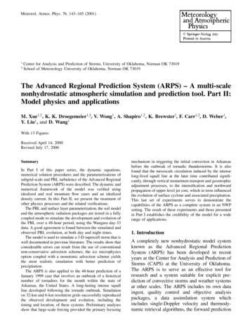
The Advanced Regional Prediction System (ARPS) Part IIcalculated by the surface layer model withstability-dependent drag coef cients and landsurface conditions predicted by the soil model.Large-scale geostrophic and thermal winds linearly interpolated between the observation timesand heights are used. A vertical grid spacing of50 m is used with a total of 230 layers. Time stepsize is 60 s for both atmospheric and the soilmodels. For the soil model, soil type used is loam,vegetation type is desert, leaf area index is 0.1,vegetation fraction is 0.05 and roughness length is0.24 m. Initial ground wetness (volumetric watercontent) is 0.1533 and that of the deep layer is0.1555.1495.2. The resultsThe vertical pro les of simulated and observedvirtual potential temperature ( v ) and speci chumidity (qv ) at various times are plotted inFig. 1. Figure 1a shows that a mixed boundarylayer is fully developed by 15 EST. A shallowsuperadiabatic layer near the surface and a layer atthe boundary layer top with negative v perturbations resulting from entrainment are seen. Bothfeatures are observed, although the model PBL isslightly deeper than the observation. By 18 EST,radiative cooling dominates at the surface and vdrops 282.7 K as compared to the observedFig. 1. Pro les of virtual potential temperature, v , (upper panel) and speci c humidity, qv , (lower panel) simulated by ARPS(left panel) and from Wangara Day 33 data (right panel)
150M. Xue et al.283.4 K. Surface cooling continued into the nightand deepens the stable boundary layer to about200 m depth, which is somewhat deeper than theobserved one. The simulated vertical temperature uxes decrease linearly with height and becomenegative in the entrainment layer, similar to theobservations (not shown).The vertical mixing dries the surface layer andmoistens in the upper PBL (Fig. 1c) in the model,again agreeing with the observation (Fig. 1d).Overall, the evolution of the simulated PBL agreesremarkably well with the observations (Clarkeet al., 1971) as well as these obtained from a high(third) order turbulence model of Andre et al.(1978).The performance of the radiation parameterization and the soil model can be illustrated bycomparing ground surface radiation, heat andmoisture uxes with observations. Figure 2 showsthat, for a 48-hour period, the model produceswell-behaved diurnal cycles in the uxes. Themagnitude and phase of the net radiation, heat andground uxes all agree well with observations.The latent heat ux is relative small in such a drycondition.The results from the above experiment, and thecomparison with the First International SatelliteLand Surface Climatology Project (ISLSCP) FieldExperiment (FIFE, Sellers et al., 1992) data (Xueet al., 1995) and with HAPEX-MOBILHY (Andreet al., 1986) data (not shown) provide reasonablevalidations for our coupled soil atmospheremodel, at least for the speci c geophysical andweather conditions. More detailed studies usingOklahoma Mesonet (Brock et al., 1995) measurements are being carried out that will test morediverse conditions.6. May 20, 1977 Del City supercellstorm simulationFig. 2. The simulated a and observed b surface uxes of netradiation (Rn ), sensible heat (H), latent heat (LE), andground heat (G) for Wangara days 33 and 34. 0Z correspondsto 9 am local timeThe 20 May 1977 Del City, Oklahoma storm is awell-documented and extensively studied tornadicsupercell storm. The morphology and evolution ofthis storm was documented in Ray et al. (1981)based on multi-Doppler radar analysis. Earlynumerical simulations by Klemp et al. (1981)simulated the general supercell morphologyreasonably well, even though the storm wasstarted from arti cial initial perturbations in ahorizontally homogeneous environment. Later, ahigh-resolution study by Klemp and Rotunno(1983) using the same sounding was able tosimulate tornadic vortex intensi cation near thetip of a surface gust front occlusion. Morerecently, this storm was simulated by Lin et al.(1993) using inhomogeneous initial conditionsderived from multiple Doppler radars, and by Xueet al. (1993) at high resolutions using the adaptivegrid re nement technique in the ARPS. Thesestudies all used Kessler-type (Kessler, 1969) warmrain microphysics, however. In this section, wepresent the results from the ARPS, using the same
The Advanced Regional Prediction System (ARPS) Part IIinitial sounding as in Klemp et al. (1981), andcompare the results against the observations andthe simulation of Klemp and Wilhelmson (1978).We also examine the impact of monotonic andpositive de nite advection schemes and the icemicrophysics on the intensity and precipitationamount of the storm. These experiments alsodemonstrate the model's ability to simulateintensive convective systems.6.1. The experimentsFor all experiments, the horizontal grid spacing is1 km and the vertical grid is stretched from 100 mat the ground to 700 m at the top. The domain is64 64 16 km3 in size. The storm was initiatedby a 4 C ellipsoidal thermal bubble centered atx 48 km, y 16 km and z 1:5 km, and withradii of 10 km in x and y directions and 1.5 km inthe vertical direction. The Orlanski (1976) openlateral boundary condition but with the columnaveraged phase speed estimation as proposed byDurran and Klemp (1983) (option 4 in ARPS) isused. A radiation condition is also used at the topboundary. A cosine instead of regular Fouriertransform is used in the condition which removesthe constraint of lateral periodicity (see Part I).151The 1.5-order turbulent kinetic energy (TKE)based subgrid-scale (SGS) turbulence option isused whose implementation follows Moeng(1984). Free-slip conditions were applied to thebottom boundary. The large and small time stepsizes are 3 s and 1 s, respectively. The stormenvironment is de ned by a sounding shown inFig. 3. A constant wind of u 3 msÿ1 andv 14 msÿ1 is subtracted from the originalsounding to keep the primary storm cell near thecenter of model grid. Fourth-order computationalmixing is applied in both horizontal and verticaldirections.The results from four experiments are presented(see Table 1). They differ in their use of advectionschemes for temperature, water species and TKEand in the choice of microphysics parameterization. In all cases, the momentum elds areadvected by fourth-order leapfrog centeredscheme. When this scheme is used (in ICE4th)to advect positive de nite elds (water species andTKE), negative values are set to zero whichconstitutes a source of error. The implementationof the monotonic FCT ( ux-corrected transport)scheme follows Zalesak (1979), with modi cations so that extrema in the advected scalar insteadof density-weighted scalar is used in the uxlimiting process. The high-order scheme used is asecond-order-in-time, fourth-order-in-space trapezoidal scheme while the lower-order scheme isupstream in space and forward in time. Thisoption was used in the density current experimentsin Part I. Experiment ICEPD uses the positivede nite scheme of Lafore et al. (1998) for theadvection of water, ice and TKE elds. Thisscheme limits the outgoing uxes
physics and/or advection schemes on the storm morphology and the amount of total precipitation from the storm. In Sect. 7, the ARPS system, including the ARPS Data Analysis System (ADAS), is applied to the 48-hour prediction of a case involving an outbreak of 56 tornadoes and the development and evolution of a long-lasting squall line. Results