Transcription
1Survey on Software Defect PredictionJaechang NamAbstractSoftware defect prediction is one of the most active research areas in software engineering. Defectprediction results provide the list of defect-prone source code artifacts so that quality assurance teamscan effectively allocate limited resources for validating software products by putting more effort on thedefect-prone source code. As the size of software projects becomes larger, defect prediction techniqueswill play an important role to support developers as well as to speed up time to market with morereliable software products.In this survey, we first introduce the common defect prediction process used in the literature and howto evaluate defect prediction performance. Second, we compare different defect prediction techniquessuch as metrics, models, and algorithms. Third, we discuss various approaches for cross-project defectprediction that is an actively studied topic in recent years. We then discuss applications on defectprediction and other emerging topics. Finally, based on this survey, we identify challenging issues forthe next step of the software defect prediction.I.I NTRODUCTIONSoftware Defect (Bug) Prediction is one of the most active research areas in software engineering [9], [31], [40], [47], [59], [75].1 Since defect prediction models provide the list ofbug-prone software artifacts, quality assurance teams can effectively allocate limited resourcesfor testing and investigating software products [40], [31], [75].We survey more than 60 representative defect prediction papers published in about ten majorsoftware engineering venues such as Transaction on Software Engineering (TSE), InternationalConference on Software Engineering (ICSE), Foundations of Software Engineering (FSE) andso on in recent ten years. Through this survey, we investigated major approaches of softwaredefect prediction and their trends.We first introduce the common software defect prediction process and several research streamsin defect prediction in Section II. Since different evaluation measures for defect prediction have1Defect and bug will be used interchangeably across this survey paper.
2been used across the literature, we present evaluation measures for defect prediction modelsin Section III. Section IV and V discusses defect prediction metrics and models used in therepresentative papers. In Section VI, we discuss about prediction granularity. Before buildingdefect prediction models, some studies applied preprocessing techniques to improve predictionperformance. We briefly investigate preprocessing techniques used in the literature in Section VII.As recent defect prediction studies have focused on cross-project defect prediction, we comparevarious cross-project defect prediction approaches in Section VIII. In the next two sections ofSection VIII, we discuss about applications using defect prediction results and emerging topics.Finally, we conclude this survey by raising challenging issues for defect prediction in Section XI.II.OVERVIEW OF S OFTWARE D EFECT P REDICTIONA. Software Defect Prediction ProcessFigure 1 shows the common process of software defect prediction based on machine learningmodels. Most software defect prediction studies have utilized machine learning techniques [3],[6], [10], [20], [31], [40], [45].The first step to build a prediction model is to generate instances from software archives suchas version control systems, issue tracking systems, e-mail archives, and so on. Each instance canrepresent a system, a software component (or package), a source code file, a class, a function(or method), and/or a code change according to prediction granularity. An instance has severalmetrics (or features) extracted from the software archives and is labeled with buggy/clean orthe number of bugs. For example, in Figure 1, instances generated from software archives arelabeled with ‘B’ (buggy), ‘C’ (clean), or the number of bugs.After generating instances with metrics and labels, we can apply preprocessing techniques,which are common in machine learning. Preprocessing techniques used in defect predictionstudies include feature selection, data normalization, and noise reduction [27], [40], [47], [63],[71]. Preprocessing is an optional step so that preprocessing techniques were not applied on alldefect prediction studies, e.g., [10], [31].With the final set of training instances, we can train a prediction model as shown in Figure 1.The prediction model can predict whether a new instance has a bug or not. The prediction forbug-proneness (buggy or clean) of an instance stands for binary classification, while that for thenumber of bugs in an instance stands for regression.
3Builda ?"New instance2"Model0".B"1"Instances withmetrics and labelsSoftwareArchivesB"C"B"1"Classification /RegressionTraining InstancesFig. 1: Common process of software defect predictionHistory of Defect Prediction1970sSimple metric andmodel (Ajiyama 71)1980sPrediction model(Regression)Fitting modelProcess metricsCyclomatic metric(McCabe 76)(Shen 85)Halstead metrics(Halstead 77)1990sPrediction model(Classification)(Munson et al. 92)2000sJust-In-Time (JIT) Prediction models(Mokus 00, Kim 08,Kamei 13,Fukushima 14)CK metrics(Chidamber222222222222222222&Kemerer 94)2(Basili 96)2010s Process Metrics Extractedfrom Software RepositoriesNagappan 05Cross-Project PredictionMoser 08 Metric CompensationHassan 09(Watanabe 08)D’Ambros 10 NN Filter (Turhan 09)Bacchelli 10 TNB (Ma 12)Bird 11 TCA (Nam 13)Lee 11Rahman 11Cross-Project Feasibility(Zimmermann 09, He 12)Practical Model and Applications Case study in Google (Lewis 13) Test case prioritization(Engstrom 10) Compensate static bug finder(Rahman 14)Other metrics Component Networkmetrics (ZimmerMann 08) Developer-Module Network(Pinzger 08) Developer Social Network(Meneely 08) Anti-pattern (Taba 13)Data Privacy(Peters 12)Personalized model(Jiang 13)Universal4Model(Zhang 13)Fig. 2: History of software defect prediction studiesB. Brief History of Software Defect Prediction StudiesFigure 2 briefly shows the history of defect prediction studies in about last 50 years. The firststudy estimating the number of defects was conducted by Akiyama in 1971 [1]. Based on the
4assumption that complex source code could cause defects, Akiyama built a simple model usinglines of code (LOC) since LOC might represent the complexity of software systems. However,LOC is too simple metric to show the complexity of systems. In this reason, MaCabe andHalstead proposed the cyclomatic complexity metric and Halstead complexity metrics in 1976and 1977 respectively [38], [18]. These metrics were very popular to build models for estimatingdefects in 1970s and the early of 1980s [13].Having said that though, the models studied in that period were not actually predictionmodel but just fitting model that investigated the correlation between metrics and the numberof defects [13]. These models were not validated on new software modules. To resolve thislimitation of previous studies, Shen et al. built a linear regression model and test the modelon the new program modules [60]. However, Munson et al. claimed that the state-of-the artregression techniques at that time were not precise and proposed a classification model thatclassify modules into two groups, high risk and low risk [43]. The classification model actuallyachieved 92% of accuracy on their subject system [43]. However, Munson et al.’s study stillhave several limitations such as no metrics for object-oriented (OO) systems and few resourcesto extract development process data. As Shen et al. pointed out at that time [60], it was notpossible to collect error fix information informally conducted by individual developers in unittesting phases.In terms of OO systems, Chidamber and Kemerer proposed several object-oriented metricsin 1994 [7] and was used by Basili et al. to predict defects in object-oriented system [4]. In1990s, version control systems were getting popular, development history was accumulated intosoftware repositories so that various process metrics were proposed from the middle of 2000s [3],[6], [9], [20], [31], [42], [45], [59].In 2000s, there had been existed several limitations for defect prediction. The first limitationwas the prediction model could be usable before the product release for the purpose of qualityassurance. However, it would be more helpful if we can predict defects whenever we changethe source code. To make this possible, Mockus et al. proposed a defect prediction model forchanges [41]. Recently, this kind of models is called as just-in-time (JIT) defect predictionmodels. JIT prediction models have been studied by other researchers in recent years [15], [25],[26].The second limitation is that it was not possible or difficult to build a prediction model for new
5projects or projects having less historical data. As use of process metrics was getting popular, thislimitation became the one of the most difficult problems in software defect prediction studies [76].To resolve this issue, researchers proposed various cross-project defect prediction models [36],[47], [67], [69]. In cross-project defect prediction, identifying cross-prediction was another issueso that Zimmermann et al. and He et al. conducted the study on cross-prediction feasibility [76],[22].The third limitation was from the question, “are the defect prediction models really helpfulin industry?”. In this direction, several studies such as case study and proposing practicalapplications have been conducted [12], [33], [57].There have been several studies following the trends of information technology as well.By using social network analysis and/or network measures, new metrics were proposed byZimmermann et al. [75], Pinzger et al [54], and Taba et al. [66]. Privacy issue of defect datasetswas also addressed by Peters et al. [53]. New concepts of prediction models have been proposedsuch as personalized defect prediction model [23] and universal model [73] recently.In the next subsection, we categorized these studies by related subtopics.C. Categories of Software Defect Prediction StudiesTable I lists the representative studies in software defect prediction. Many research studiesin a decade have focused on proposing new metrics to build prediction models. Widely studiedmetrics are source code and process metrics [56]. Source code metrics measure how source codeis complex and the main rationale of the source code metrics is that source code with highercomplexity can be more bug-prone. Process metrics are extracted from software archives suchas version control systems and issue tracking systems that manage all development histories.Process metrics quantify many aspects of software development process such as changes ofsource code, ownership of source code files, developer interactions, etc. Usefulness of processmetrics for defect prediction has been proved in many studies [20], [31], [45], [56].As introduced in Section II-A, most defect prediction studies are conducted based on statisticalapproach, i.e. machine learning. Prediction models learned by machine learning algorithms canpredict either bug-proneness of source code (classification) or the number of defects in sourcecode (regression). Some research studies adopted recent machine learning techniques such asactive/semi-supervised learning to improve prediction performance [34], [68]. Kim et al. proposed
6TABLE I: Representative studies in software defect ],[10],Popularity[3],Within/CrossAuthorship [55], Ownership [6], MIM [31]), Networkmeasure [39], [54], [75], Antipattern e/Semi-supervisedlearning [34], [68], BugCache [29]Finer prediction granularityChange classification [26], Method-level prediction [21]PreprocessingFeature selection/extraction [63], [45], Normalization [40], [47], Noise handling [27], [71]Transfer learningMetric compensation [69], NN Filter [67], TNB [36],CrossTCA [47]FeasibilityDecision Tree [76], [22]BugCache algorithm, which utilizes locality information of previous defects and keeps a list ofmost bug-prone source code files or methods [29]. BugCache algorithm is a non-statistical modeland different from the existing defect prediction approaches using machine learning techniques.Researchers also focused on finer prediction granularity. Defect prediction models tried toidentify defects in system, component/package, or file/class levels. Recent studies showed thepossibility to identify defects even in module/method and change levels [21], [26]. Finer granularity can help developers by narrowing the scope of source code review for quality assurance.Proposing preprocessing techniques for prediction models is also an important research branchin defect prediction studies. Before building a prediction model, we may apply the followingtechniques: feature selection [63], normalization [40], [47], and noise handling [27], [71]. Withthe preprocessing techniques proposed, prediction performance could be improved in the relatedstudies [27], [63], [71].Researchers also have proposed approaches for cross-project defect prediction. Most representative studies described above have been conducted and verified under the within-predictionsetting, i.e. prediction models were built and tested in the same project. However, it is difficult for
7new projects, which do not have enough development historical information, to build predictionmodels. Representative approaches for cross defect prediction are metric compensation [69],Nearest Neighbour (NN) Filter [67], Transfer Naive Bayes (TNB) [36], and TCA [47]. Theseapproaches adapt a prediction model by selecting similar instances, transforming data values, ordeveloping a new model [67], [47], [36], [69].Another interesting topic in cross-project defect prediction is to investigate feasibility ofcross-prediction. Many studies confirmed that cross-prediction is hard to achieve; only fewcross-prediction combinations work [76]. Identifying cross-prediction feasibility will play a vitalrole for cross-project defect prediction. There is a couple of studies regarding cross predictionfeasibility based on decision trees [76], [22]. However their decision trees were verified only inspecific software datasets and were not deeply investigated [76], [22].III.E VALUATION M EASURESFor defect prediction performance, various measures have been used in the literature.A. Measures for ClassificationTo measure defect prediction results by classification models, we should consider the followingprediction outcomes first: True positive (TP): buggy instances predicted as buggy. False positives (FP): clean instances predicted as buggy. True negative (TN): clean instances predicted as clean. False negative (FN): buggy instances predicted as clean.With these outcomes, we can define the following measures, which are mostly used in thedefect prediction literature.1) False positive rate (FPR): False positive rate is also know as probability of false alarm(PF) [40]. PF measures how many clean instances are predicted as buggy among all cleaninstances.FPTN FP(1)
82) Accuracy:TP TNTP FP TN FN(2)Accuracy considers both true positives and true negatives over all instances. In other words,accuracy shows the ratio of all correctly classified instances. However, accuracy is not propermeasure particularly in defect prediction because of class imbalance of defect prediction datasets.For example, average buggy rate of PROMISE datasets used by Peters et al. [53] is 18%. If weassume a prediction model that predicts all instances as clean, the accuracy will be 0.82 althoughno buggy instances are correctly predicted. This does not make sense in terms of defect predictionperformance. Thus, accuracy has not been not recommended for defect prediction [58]3) Precision:TPTP FP(3)4) Recall: Recall is also know as probability of detection (PD) or true positive rate (TPR) [40].Recall measures correctly predicted buggy instances among all buggy instances.TPTP FN(4)5) F-measure: F-measure is a harmonic mean of precision and recall [31].2 (P recision Recall)P recision Recall(5)Since precision and recall have trade-off, f-measure has been used in many papers [27], [31],[47], [56], [71].6) AUC: AUC measures the area under the receiver operating characteristic (ROC) curve.The ROC curve is plotted by PF and PD together. Figure 3 explains about a typical ROC curve.PF and PD vary based on threshold for prediction probability of each classified instance. Bychanging the threshold, we can draw a curve as shown in Figure 3. When the model gets better,the curve tends to be close to the point of PD 1 and PF 0. Thus, AUC of the perfect modelwill have “1”. For a random model, the curve will be close to the straight line from (0,0) to(1,1) [40], [58]. AUC with 0.5 is regarded as the random prediction [58]. Other measures such asprecision and recall can vary according to prediction threshold values. However, AUC considersprediction performance in all possible threshold values. In this reason, AUC is a stable measureto compare different prediction models [58].
MENZIES ET AL.: DATA MINING STATIC CODE ATTRIBUTES TO LEARN DEFECT PREDICTORS9Fig. 9. A ROC sheet assessin{A,B,C,D} shows the number ofROC sheet. The bal (or balanceFig. 8. Regions of a typical ROC curve.Fig. 3: A typical ROC curve [40]predictor more often. This,order). Randomizing the order of the inputs defends against false alarms.P f and pd can be calcorder effects.These M ! N studies implement a holdout study which, as Fig. 9. Consider a predictoargued above, is necessary to properly assess the value of a some signal, either triggers7) AUCEC: Area under cost-effectiveness curve (AUCEC) is a defect prediction whethermeasure conor not the signallearned predictor. Holdout studies assess a learned predictorshowsfoursidering lines of usingcode (LOC)be inspectedor it.testedqualitystudiesassurancedata nottousedto generateSuchbyholdoutareteamsthe or developers. interesting sitpreferred evaluation method when the goal is to produce silent when the signal is abThe idea of cost-effectiveness for defect prediction models is proposed by Arisholmet al. [2]. if the predicAlternatively,predictors intended to predict future events [23].signal oris actually abseCost-effectiveness representshow manydefectsbe foundamongtop n%LOCtheinspectedThe 10 ! 10-waystudywas subsets ofthe canattributesin defectsthe ordertested. In other words,if adifferentcertain predectionmodelfind morewith less inspectingIf the predictor registerssuggested by InfoGain (2). In the innermost loop of theinterest.In one case, the prand testing st-effectivenessofthe modelsome method was applied to some data set. As shownin the third to the last line of Fig. 7, these methods were some the signal. This probabilityis higher.detected signals, true positcombination of filter, attributes’, and learner.Figure 4 shows cost-effectiveness curves as examples [59]. The x-axis represents the percentprobability detection ¼age of LOC 9].Intheleftside of7 ASSESSING PERFORMANCE(Note that pd is also callethe figure, three Theexamplecurves areofplotted.Let assumeO, P, wasand R, probabilityrepresent theof a false alarmperformancethe learnerson thethe curves,MDP dataassessedusingreceiver-operatorFormally,a underno signalwas present to aloptimal, practical,and randommodels,respectively(ROC)[59]. Ifcurves.we considerthe areathe curve,defect predictor hunts for a signal that a software module isfalse althe optimal modelwill havethe highestcomparingothermodels[59]. In case ofprobabilitythedefectprone.Signal AUCECdetectiontheory to[42]offersROCcurves asanalysismethodfor assessingdifferentrandom model, AUCECwillanbe 0.5.The higherAUCECof the optimalmodel meansthat weFor convenience,we say thpredictors. A typical ROC curve is shown in Fig. 8. Thecan find more defectsinspectingor testingLOC than[59].notPf ¼ 1y-axis byshowsprobabilityof lessdetection(pd) otherand modelsthe x-axisshows probabilityof thefalsewholealarms(pf).the[59]. In the rightHowever, consideringAUCEC fromLOCmayBynotdefinition,make senseFig. 9 also lets us define theROC curve must pass through the points pf ¼ pd ¼ 0 andthe percentageside of Figure 4,pfthecost-effectivenesscurvesthe models,and P2,are identicalso that of true nega¼ pd¼ 1 (a predictorthatofnevertriggersP1nevermakesfalse LOCalarms;a predictorthatgivealwaystriggers insightalways[59]. Havingaccuracyconsidering the wholefor AUCECdoes notany meaningfulsaid¼ acc ¼ ðAgenerates false alarms). Three interesting trajectories conthat, if we set a threshold as top 20% of LOC, the model P2 has higher AUCEC thanR and as percentaIf reportednect these points:range1. A straight line from (0, 0) to (1, 1) is of little interest0 ' acc%; pdsince it offers no information; i.e., the probability of apredictor firing is the same as it being silent.Ideally, we seek predic2. Another trajectory is the negative curve that bends pd percent, and notPf percenaway from the ideal point. Elsewhere [14], we haveNote that maximizing a
10O10010020%cache that cSo we adoptaucec20 .P1P275RPercent of Bugs FoundPercent of Bugs FoundP502575R503. EXPE25In this secour experim3.1ReviSource coversion histocommits to eFigure 1: Cost Effectiveness Curve. On the left, O isCost-effectivenesssuch as a timthe optimal, RFig.is 4:random,and Pcurveis a[59]possible, practical,log message.predictor model. On the right, we have two differentan author, amodels P1 and P2, with the same overall performance,Git as our vbut P2 is better when inspecting 20% of the lines or less.P2 [59]. In this reason, we need to consider a particularthreshold for the percentage of LOC toability to trcode.255075Percent of LOC100255075Percent of LOC100use AUCEC as a prediction measure [59].3.2 Bugthis procedure would allow us to inspect just a few lines ofB. Measuresfor toRegressionBugs arecodefind most of the defects. If the algorithm performstracking syspoorly and/or the defects are uniformly distributed in theTo measure defect prediction results from regression models, measures based on correlationor fixed bycode, we would expect to inspect most of the lines before edictedbugsofinstanceshavebeenusedinopening dateall the defects. The CE curve (see Figure 1, left side)description,many defect[3], [46], [62],judge[75]. Therepresentativealgorithms;measures are Spearman’sis predictiona harsh papersbut meticulousof predictionitthecorrelation,proportionof identifiedfaultsbetweencorrelation,plotsPearsonR2 andtheir variations[3], (a[46],number[62], [75].These measuresresearch, weto be a bug.0 and 1) found against the proportion of the lines of codealso has been used for correlation analysis between metric values and the number of bugs [75].Our study(also between 0 and 1) inspected. It is a way to evaluate aspecific revisproposed inspection ordering. With a random ordering (theC. DiscussiononMeasuresrevision. Wecurve labeled R on the left side of Figure 1) and/or defectsWe scan for kuniformly scattered throughout the code, the CE curve is theFigure 5 shows the count of evaluation measures used in the representative defect predictioncommit log tdiagonal y x line. At file-granularity, the optimal orderingpapers for eisthemostfrequentlyusedmeasurebug identifieO in the Figure 1 left) places the smallest, mostfor defect defectiveclassification.filesSincefirst,there andare trade-offbetweenprecisionand recall,comparing dif-to the issuethe curveclimbsrapidly,quicklyrisingabovethe modelsy x haveline.highA practicalalgorithma versaidentifiers arferent modelsare wellnot easyas someprecision butlow recall hasand viceto see whethCE curve (labeled P in the Figure 1 left) that falls below thefor other models. Since f-measure is a harmonic mean of precision and recall and provides oneits status choptimal ordering, but remains usefully above the y x line.manually insThe CE curve represents a variety of operating choices:as possible.one can choose an operating point along this curve, inspectrevision. Wemore or fewer lines of code and find more or fewer defects.from BachmThus, to jointly capture the entire set of choices affordedby a particular prediction algorithm, one typically uses the3.3Bug-
Measures02468101211PFAccuracyPrecisionRecall (PD)F-measureAUCAUCECFig. 5: Count of evaluation measures used in the representative defect prediction papers forclassification.single score as prediction performance, f-measure has been used to compare different predictionmodels in many defect prediction papers [27], [31], [47], [53], [58], [61].However, f-measure varies by different thresholds (cutoffs) for prediction probability of aninstance. When a model predicts an instance as buggy, it provides prediction probability thatrepresents if the instance is buggy. Lessmann et al. pointed out that what thresholds were usedin evaluation usually overlooked in the defect prediction literature so that it led to inconsistentprediction results across defect prediction papers [32].To overcome the limitation of f-measures, researchers also used other measures such as AUCand AUCEC that are independent from the thresholds [16], [32], [58], [65]. Particularly, AUCECrecently used a lot by Rahmann et al. since AUCEC could be a good measure to evaluateprediction models in the view of practical use of models [56], [58], [59].IV.D EFECT P REDICTION M ETRICSDefect prediction metrics play the most important role to build a statistical prediction model.Most defect prediction metrics can be categorized into two kinds: code metrics and processmetrics. Code metrics are directly collected existing source code while process metrics arecollected from historical information archived in various software repositories such as versioncontrol and issue tracking systems.
12A. Code metricsCode metrics also known as product metrics measure complexity of source code. Its groundassumption is that complexity source is more bug-prone. To measure code complexity, researchersproposed various metrics.TABLE II: Representative code metricsCode MetricsSize [1]Halstead [18]McCabe [38], [48]CK [7], [4]OO �94,’96JSS’94The size metrics measure “volume, length, quantity, and overall magnitude of software products” [8]. The representative of size metrics is lines of code (LOC). To our knowledge, Akiyama’smodel was the earliest study to predict defects using LOC [1]. Afterwards, LOC was used inmost defect prediction papers to build a model [10], [21], [31], [40], [61], [65].Halstead proposed several size metrics based on the number of operators and operands [18].The proposed metrics are program vocabulary, length, volume, difficult, effort, and time [18].Most metrics are related to size or quantity. Halstead metrics has been used popularly in manystudies [40], [65], [67].McCabe proposed the cyclomatic metric to represent complexity of software products [38].Cyclomatic metric is computed by the number of nodes, arcs and connected components incontrol flow graphs of source code. This metric represents how much control paths are complex.Since McCabe’s cyclomatic metric measure the complexity of source code structure, its characteristic is inherently different from size and Halstead metrics that measure volume and quantityof source code. Ohlsson and Alberg adopted McCabe’s cyclomatic metric to predict fault-pronemodules in telephone switched [48] and other defect prediction studies [32], [40], [42], [47],[65], [67] also used McCabe’s cyclomatic metric to build a prediction model.Since object-oriented programming is getting popular, code metrics for object-oriented languages have proposed to improve development process. The representative metrics for objectoriented programs are Chidamber and Kemerer (CK) metrics [7]. Table III lists CK metrics.The CK metrics were designed from the characteristics from object-oriented languages such as
13inheritance, coupling, and cohesion [7]. Basili et al. [4] validated if it is possible to build adefect prediction model using the CK metrics. After that, many studies include CK metrics tobuild prediction models [3], [10], [24], [27], [31], [50], [71].TABLE III: CK metrics [7]NameDescriptionWMCWighted methods per classDITDepth of inheritance treeNOCNumber of childrenCBOCoupling between object classesRFCResponse for a classLCOMLack of cohesion in methodsBesides the CK metrics, other object-oriented (OO) metrics based on volume and quantity ofsource code, have been proposed as well [11]. As size metrics, the OO metrics simply counts thenumber of instance variables, methods, and etc. as shown in Table IV. Many defect predictionstudies for object-oriented programs have used the OO metrics to build prediction models [10],[27], [31], [50], [71], [74], [75].B. Process metricsTable V lists seven representative process metrics. In this section, we briefly introduce themetrics and their design concepts.1) Relative code change churn: Nagappan and ball [45] proposed 8 relative code churn metrics(M1-M8) measuring the amount of code changes [45]. For example, M1 metric is computed bychurned LOC (the accumulative number of deleted and added lines between a base version and anew version of a source file) divided by Total LOC [45]. Other metrics (M2-M8) consider variousnormalized changes such as deleted LOC divided by total LOC, file churned (the number ofchanged files in a component) divided by file count, and so on [45]. In case study by Nagappanand ball, the relative churn metrics is proved as
Software defect prediction is one of the most active research areas in software engineering. Defect prediction results provide the list of defect-prone source code artifacts so that quality assurance teams can effectively allocate limited resources for validating software products by putting more effort on the