Transcription
RADIOSS THEORY MANUAL14.0 version – July 2015Large Displacement Finite Element AnalysisPART 2Altair Engineering, Inc., World Headquarters: 1820 E. Big Beaver Rd., Troy MI 48083-2031 USAPhone: 1.248.614.2400 Fax: 1.248.614.2411 www.altair.com info@altair.com
RADIOSS THEORY Version 14.0CONTENTSCONTENTS9.0 MATERIAL LAWS39.1 ISOTROPIC ELASTIC MATERIAL9.2 COMPOSITE AND ANISOTROPIC MATERIALS699.2.1 FABRIC LAW FOR ELASTIC ORTHOTROPIC SHELLS (LAWS 19 AND 58)9.2.2 NONLINEAR PSEUDO-PLASTIC ORTHOTROPIC SOLIDS (LAWS 28, 50 AND 68)9.2.3 HILL’S LAW FOR ORTHOTROPIC PLASTIC SHELLS (LAW 72)9.2.4 ELASTIC-PLASTIC ORTHOTROPIC COMPOSITE SHELLS9.2.5 ELASTIC-PLASTIC ORTHOTROPIC COMPOSITE SOLIDS9.2.6 ELASTIC-PLASTIC ANISOTROPIC SHELLS (BARLAT’S LAW)9.3 ELASTO-PLASTICITY OF ISOTROPIC MATERIALS9.3.1 JOHNSON-COOK PLASTICITY MODEL (LAW 2)9.3.2 ZERILLI-ARMSTRONG PLASTICITY MODEL (LAW 2)9.3.3 COWPER-SYMONDS PLASTICITY MODEL (LAW 44)9.3.4 ZHAO PLASTICITY MODEL (LAW 48)9.3.5 TABULATED PIECEWISE LINEAR AND QUADRATIC ELASTO-PLASTIC LAWS(LAWS 36 AND 60)9.3.6 DRUCKER-PRAGER CONSTITUTIVE MODEL (LAWS 10 AND 21)9.3.7 BRITTLE DAMAGE FOR JOHNSON-COOK PLASTICITY MODEL (LAW 27)9.3.8 BRITTLE DAMAGE FOR REINFORCED CONCRETE MATERIALS (LAW 24)9.3.9 DUCTILE DAMAGE MODEL9.3.10 DUCTILE DAMAGE MODEL FOR POROUS MATERIALS (GURSON LAW 52)9.3.11 CONNECT MATERIALS (LAW 59)9.4 VISCOUS MATERIALS9.4.1 BOLTZMANN VISCOELASTIC MODEL (LAW 34)9.4.2 GENERALIZED KELVIN-VOIGT MODEL (LAW 35)9.4.3 TABULATED STRAIN RATE DEPENDENT LAW FOR VISCOELASTIC MATERIALS (LAW 38)9.4.4 GENERALIZED MAXWELL-KELVIN MODEL FOR VISCOELASTIC MATERIALS (LAW 40)9.4.5 VISCO-ELASTO-PLASTIC MATERIALS FOR FOAMS (LAW 33)9.4.6 HYPER VISCO-ELASTIC LAW FOR FOAMS (LAW 62)9.5 MATERIALS FOR HYDRODYNAMIC ANALYSIS9.5.1 JOHNSON COOK LAW FOR HYDRODYNAMICS (LAW 4)9.5.2 HYDRODYNAMIC VISCOUS FLUID LAW (LAW 6)9.5.3 ELASTO-PLASTIC HYDRODYNAMIC MATERIAL (LAW 3)9.5.4 STEINBERG-GUINAN MATERIAL (LAW 49)9.6 VOID MATERIAL (LAW 0)9.7 FAILURE MODEL9.7.1 JOHNSON-COOK FAILURE MODEL9.7.2 WILKINS FAILURE CRITERIA9.7.3 TULER-BUTCHER FAILURE CRITERIA9.7.4 FORMING LIMIT DIAGRAM FOR FAILURE (FLD)9.7.5 SPALLING WITH JOHNSON-COOK FAILURE MODEL9.7.6 BAO-XUE-WIERZBICKI FAILURE MODEL9.7.7 STRAIN FAILURE MODEL9.7.8 SPECIFIC ENERGY FAILURE MODEL9.7.9 XFEM CRACK INITIALIZATION FAILURE 1
Chapter9MATERIALS30-July-2015
RADIOSS THEORY Version 14.0MATERIALS9.0 MATERIAL LAWSA large variety of materials is used in the structural components and must be modeled in stress analysis problems.For any kind of these materials a range of constitutive laws is available to describe by a mathematical approachthe behavior of the material. The choice of a constitutive law for a given material depends at first to desired qualityof the model. For example, for standard steel, the constitutive law may take into account the plasticity, anisotropichardening, the strain rate, and temperature dependence. However, for a routine design maybe a simple linear elasticlaw without strain rate and temperature dependence is sufficient to obtain the needed quality of the model. This isthe analyst design choice. On the other hand, the software must provide a large constitutive library to providemodels for the more commonly encountered materials in practical applications.RADIOSS material library contains several distinct material laws. The constitutive laws may be used by the analystfor general applications or a particular type of analysis. You can also program a new material law in RADIOSS.This is a powerful resource for the analyst to code a complex material model.Theoretical aspects of the material models that are provided in RADIOSS are described in this chapter. Theavailable material laws are classified in Table 9.0.1. This classification is in complementary with those ofRADIOSS input manual. The reader is invited to consult that one for all technical information related to thedefinition of input data.30-July-20153
RADIOSS THEORY Version 14.0GroupElasto-plasticity MaterialsHyper and Visco-elastic30-July-2015MATERIALSTable 9.0.1 Material law descriptionModel descriptionLaw number inRADIOSS (MID)Johnson-Cook(2)Zerilli-Armstrong(2)von Mises isotropic hardening withpolynomial pressure(3)Johnson-Cook(4)Gray model(16)Ductile damage for solids andshells(22)Ductile damage for solids(23)Aluminum, glass, etc.(27)Hill(32)Tabulated piecewise an(49)Ductile damage for porousmaterials, Gurson(52)Foam model(53)3-Parameter Barlat(57)Tabulated quadratic in strain rate(60)Hänsel model(63)Ugine and ALZ pic Hill(72)Thermal Hill Orthotropic(73)Thermal Hill Orthotropic 3D(74)Semi-analytical elasto-plastic(76)Yoshida-Uemori(78)Brittle Metal and Glass(79)High strength steel(80)Swift and Voce elastio-plasticMaterial(84)Closed cell, elasto-plastic foam(33)Boltzman(34)Generalized Kelvin-Voigt(35)Tabulated law(38)Generalized Maxwell-Kelvin(40)4
RADIOSS THEORY Version 14.0GroupComposite and FabricConcrete and RockHoneycombMulti-Material, Fluid andExplosive MaterialConnections MaterialsOther Materials30-July-2015MATERIALSModel descriptionLaw number inRADIOSS (MID)Ogden-Mooney-Rivlin(42)Hyper visco-elastic(62)Tabulated input for Hyper-elastic(69)Tabulated law - hyper visco-elastic(70)Tabulated law - visco-elastic foam(77)Ogden material(82)Tsai-Wu formula for solid(12)Composite Solid(14)Composite Shell Chang-Chang(15)Fabric(19)Composite Shell(25)Fabric(58)Drucker-Prager for rock or concreteby polynominal(10)Drucker-Prager for rock or concrete(21)Reinforced concrete(24)Drücker-Prager with cap(81)Honeycomb(28)Crushable foam(50)Cosserat Medium(68)Jones Wilkins Lee model(5)Hydrodynamic viscous(6)Hydrodynamic viscous with k-ε(6)Boundary element(11)Boundary element with k-ε(11)ALE and Euler formulation(20)Hydrodynamic bi-material liquidgas material(37)Lee-Tarver material(41)Viscous fluid with LES subgridscale viscosity(46)Solid, liquid, gas and explosives(51)Predit rivets(54)Connection material(59)Advanced connection material(83)Fictitious(0)Hooke(1)Purely thermal material(18)5
RADIOSS THEORY Version 14.0MATERIALSGroupModel descriptionLaw number inRADIOSS (MID)SESAM tabular EOS, used with aJohnson-Cook yield criterion(26)Porous material(75)GAS materialGAS (-)User material(29 31)9.1 Isotropic Elastic MaterialTwo kinds of isotropic elastic materials are considered: Hooke’s law for linear elastic materials, Ogden and Mooney-Rivlin laws for nonlinear elastic materials.These material laws are used to model purely elastic materials, or materials that remain in the elastic range. TheHooke’s law requires only two values to be defined; the Young's or elastic modulus E, and Poisson's ratio, υ .The law represents a linear relation between stress and strain.The Ogden’s law is applied to slightly compressible materials as rubber or elastomer foams undergoing largedeformation with an elastic behavior [34]. The strain energy W is expressed in a general form as a function ofW (λ1 , λ2 , λ3 ) :W (λ1, λ 2 , λ 3 ) pµpαp(λαp1αα) λ 2p λ 3 p 3 K(J 1) 22EQ. 9.1.0.1where λi , ith principal stretch ( λi 1 ε i , ε i being the ith principal engineering strain), J λ1 λ2 λ3 , relative1 3ρvolume: J 0 , λi J λ i is the deviatoric stretch, and, α p and µ p material constants.ρThis law is very general due to the choice of coefficientαpandµp .For an incompressible material, we have J 1. For uniform dilatation:λ1 λ2 λ3 λEQ. 9.1.0.2The strain energy function can be decomposed into deviatoric and spherical parts:W W ( λ1, λ2 , λ3 ) U(J)EQ. 9.1.0.3With:W (λ1 , λ2 , λ3 ) pµp αααλ λ2 λ3 3αp 1U(J ) (ppp)K( J 1) 22The stress corresponding to this strain energy is given by:σi 30-July-2015λi WJ λiEQ. 9.1.0.46
RADIOSS THEORY Version 14.0MATERIALSwhich can be written as:σi Sinceλiλ i W λ i 3 W λ j U J J λ iJ j 1 λ j λ i J λ i EQ. 9.1.0.5 λ j 2 13 λ j 1 13 λ j Jfor i j, EQ. 9.1.0.5 is simplified to: J and J for i j and J λi 3 λi 3λi λiσi 1 W 1 3 W U λj JλiJ λi 3 j 1 λ j J EQ. 9.1.0.6For which the deviator of the Cauchy stress tensor, and the pressure would be:si p 1J W 1 3 W λi λj λ3 j 1 λ j i EQ. 9.1.0.71 3 Uσj 3 j 1 JEQ. 9.1.0.8The only deviatoric stress above is retained, and the pressure is computed independently as follows:p K f bulk ( J ) ( J 1)EQ. 9.1.0.9where f bulk a user-defined function related to the bulk modulus K:K µ µ µ2(1 υ )3(1 2υ ) µpEQ. 9.1.0.10 α ppEQ. 9.1.0.112being the ground shear modulus, andυthe Poisson's ratio.Note: For an incompressible material you havetoo small time steps in explicit codes.30-July-2015υ 0.5. However,υ 0.495is a good compromise to avoid7
RADIOSS THEORY Version 14.0MATERIALSMooney-Rivlin material law admits two basic assumptions: The rubber is incompressible and isotropic in unstrained state, The strain energy expression depends on the invariants of Cauchy tensor.The three invariants of the Cauchy-Green tensor are:I1 λ1 λ2 λ3222I 2 λ1 λ2 λ2 λ3 λ3 λ1222222EQ. 9.1.0.14I 3 λ1 λ2 λ3 1 for incompressible material222The Mooney-Rivlin law gives the closed expression of strain energy as:W C10 (I1 3) C01 (I 2 3)with:EQ. 9.1.0.15µ1 2 C10µ 2 2 C01α1 2α 2 2EQ. 9.1.0.16The model can be generalized for a compressible material.Viscous effects are modeled through the Maxwell model:G1η1G2η2G3η3G4η4Maxwell modelWhere, the shear modulus of the hyper-elastic law µ is exactly the long-term shear modulus G .τi are relaxation times:τi ηiGiRate effects are modeled through visco-elasticity using convolution integral using Prony series. Thiscorresponds to extension of small deformation theory to finite deformation.This viscous stress is added to the elastic one.30-July-20158
RADIOSS THEORY Version 14.0MATERIALSThe visco-Kirchoff stress is given by:mti 10τ Gi ev t sτi[]ddev ( F F T ) dsdsWhere, m is the order of the Maxwell model, F is the deformation gradient matrix, ,EQ. 9.1.0.17 1F J 3 F anddev ( F F T ) denotes the deviatoric part of tensor F F T .The viscous-Cauchy stress is written as:1σ v (t) τ v (t)JEQ. 9.1.0.189.2 Composite and Anisotropic MaterialsThe orthotropic materials can be classified into following cases: Linear elastic orthotropic shells as fabric Nonlinear orthotropic pseudo-plastic solids as honeycomb materials Elastic-plastic orthotropic shells Elastic-plastic orthotropic compositesThe purpose of this section is to describe the mathematical models related to composite and orthotropic materials.9.2.1 Fabric law for elastic orthotropic shells (laws 19 and 58)Two elastic linear models and a nonlinear model exist in RADIOSS.9.2.1.1 Fabric linear law for elastic orthotropic shells (law 19)A material is orthotropic if its behavior is symmetrical with respect to two orthogonal plans. The fabric law enablesto model this kind of behavior. This law is only available for shell elements and can be used to model an airbagfabric. Many of the concepts for this law are the same as for law 14 which is appropriate for composite solids. Ifaxes 1 and 2 represent the orthotropy directions, the constitutive matrix C is defined in terms of material properties: 1 E 11 υ12 E11 C 1 0 0 0 30-July-2015 υ 21000001G120001G23000E221E22 0 0 0 0 1 G31 EQ. 9.2.1.19
RADIOSS THEORY Version 14.0MATERIALSwhere the subscripts denote the orthotropy axes. As the matrix C is symmetric:υ12E11 υ 21EQ. 9.2.1.2E22Therefore, six independent material properties are the input of the material:E 11 Young's modulus in direction 1E 22 Young's modulus in direction 2υ 12 Poisson's ratioG 12 , G 23 , G 31 Shear moduli for each directionThe coordinates of a global vectorV is used to define direction 1 of the local coordinate system of orthotropy.The angle Φ is the angle between the local direction 1 (fiber direction) and the projection of the global vectoras shown in Figure 9.2.1.VFigure 9.2.1 Fiber Direction OrientationThe shell normal defines the positive direction for Φ . Since fabrics have different compression and tensionbehavior, an elastic modulus reduction factor, RE, is defined that changes the elastic properties of compression.The formulation for the fabric law has a σ 11 reduction if σ 11 0 as shown in Figure 9.2.2.Figure 9.2.2 Elastic Compression Modulus Reduction30-July-201510
RADIOSS THEORY Version 14.0MATERIALS9.2.1.2 Fabric nonlinear law for elastic anisotropic shells (law 58)This law is used with RADIOSS standard shell elements and anisotropic layered property (type 16). The fiberdirections (warp and weft) define the local axes of anisotropy. Material characteristics are determinedindependently in these axes. Fibers are nonlinear elastic and follow the equation:σ Eε Bε 2 , withdσ 0dεEQ. 9.2.1.3The shear in fabric material is only supposed to be function of the angle between current fiber directions (axes ofanisotropy):τ G0 tan(α ) τ 0ifτ G tan(α ) G A τ 0ifα αTEQ. 9.2.1.4α αTandG A (G0 G ) tan(αT ) ,G GT1 tan 2 (α T )withτ 0 G0 tan(α 0 )αT , and G0 is a shear modulus at αG0 0, the default value is calculated to avoid shear modulus discontinuity at αT : G0 G.WhereαTis a shear lock angle, GT is a tangent shear modulus at 0. IfFigure 9.2.4 Elastic Compression Modulus Reductionweftαwarpφα0is an initial angle between fibers defined in the shell property (type 16).The warp and weft fiber are coupled in tension and uncoupled in compression. But there is no discontinuitybetween tension and compression. In compression only fiber bending generates global stresses. Figure 9.2.5illustrates the mechanical behavior of the structure.30-July-201511
RADIOSS THEORY Version 14.0MATERIALSFigure 9.2.5 Local frame definitionWarp traction (free in weft direction)Warp compression (no traction in weft)A local micro model describes the material behavior (Figure 9.2.6). This model represents just ¼ of a warp fiberwave length and ¼ of the weft one. Each fiber is described as a nonlinear beam and the two fibers are connectedwith a contacting spring. These local nonlinear equations are solved with Newton iterations at membraneintegration point.Figure 9.2.6 Local frame definitionWeftWarpTraction(fiber coupling)Compression(no coupling)9.2.2 Nonlinear pseudo-plastic orthotropic solids (laws 28, 50 and68)9.2.2.1 Conventional nonlinear pseudo-plastic orthotropic solids (laws 28and 50)These laws are generally used to model honeycomb material structures as crushable foams. The microscopicbehavior of this kind of materials can be considered as a system of three independent orthogonal springs. Thenonlinear behavior in orthogonal directions can then be determined by experimental tests. The behavior curves areinjected directly in the definition of law. Therefore, the physical behavior of the material can be obtained by asimple law. However, the microscopic elasto-plastic behavior of a material point cannot be represented bydecoupled unidirectional curves. This is the major drawback of the constitutive laws based on this approach. Thecell direction is defined for each element by a local frame in the orthotropic solid property. If no property set isgiven, the global frame is used.30-July-201512
RADIOSS THEORY Version 14.0MATERIALSFigure 9.2.7 Local frame definitionThe Hooke matrix defining the relation between the stress and strain tensors is diagonal, as there is no Poisson'seffect: σ 11 E11 σ 0 22 σ 33 0 σ 12 0 σ 23 0 σ 31 00E22000E330000000000G1200G230000 ε11 ε 22 ε 33 0 ε12 0 ε 23 G31 ε 31 EQ. 9.2.2.1E112EQ. 9.2.2.2000An isotropic material may be obtained if:E11 E22 E33 and G12 G23 G31 Plasticity may be defined by a volumic strain or strain dependent yield curve (Figure 9.2.8). The input yield stressfunction is always positive. If the material undergoes plastic deformation, its behavior is always orthotropic, as allcurves are independent to each other.Figure 9.2.8 Honeycomb typical constitutive curveThe failure plastic strain may be input for each direction. If the failure plastic strain is reached in one direction,the element is deleted. The material law may include strain rate effects (law 50) or may not (law 28).30-July-201513
RADIOSS THEORY Version 14.0MATERIALS9.2.2.2 Cosserat medium for nonlinear pseudo-plastic orthotropic solids(law 68)Conventional continuum mechanics approaches cannot incorporate any material component length scale.However, a number of important length scales as grains, particles, fibers, and cellular structures must be taken intoaccount in a realistic model of some kinds of materials. To this end, the study of a microstructure material havingtranslational and rotational degrees-of-freedom is underlying. The idea of introducing couple stresses in thecontinuum modelling of solids is known as Cosserat theory which returns back to the works of brothers Cosseratin the beginning of 20th century [110]. A recent renewal of Cosserat mechanics is presented in several works ofForest et al [111], [112], [113], and [114]. A short summary of these publications is presented in this section.Cosserat effects can arise only if the material is subjected to non-homogeneous straining conditions. A Cosseratmedium is a continuous collection of particles that behave like rigid bodies. It is assumed that the transfer of theinteraction between two volume elements through surface element dS occurs not only by means of a traction andshear forces, but also by moment vector as shown in Figure 9.2.9.Figure 9.2.9 Equilibrium of Cosserat volume elementµ32σ 22 σ12σ 21µ3121σ 11L σ 11µ31Surface forces and couples are then represented by the generally non-symmetrical force-stress and couple-stresstensors σ ij and µij (units MPA and MPa-m):ti σ ij n j ;mi µ ij n jEQ. 9.2.2.3The force and couple stress tensors must satisfy the equilibrium of momentums:σ ij , j f i ρuɺɺiµij , j ε iklσ kl ci IφɺɺiWhere, f i are the volume forces, ci volume couples,the signature of the perturbation (i,k,l).EQ. 9.2.2.4ρ mass density, I the isotropic rotational inertia and ε iklIn the often used couple-stress, the Cosserat micro-rotation is constrained to follow the material rotation given bythe skew-symmetric part of the deformation gradient:12φi ε ijk u j ,kEQ. 9.2.2.5The associated torsion-curvature and couple stress tensors are then traceless. If a Timoshenko beam is regarded asa one-dimensional Cosserat medium, constraint EQ. 9.2.2.5 is then the counterpart of the Euler-Bernoulliconditions.30-July-201514
RADIOSS THEORY Version 14.0MATERIALSThe resolution of the previous boundary value problem requires constitutive relations linking the deformation andtorsion-curvature tensors to the force- and couple-stresses. In the case of linear isotropic elasticity, we have:σ ij λekk δ ij 2 µ eijSymm. 2 µc eijSkew Symm.EQ. 9.2.2.6µij α k kkδ ij 2β κ ijSymm. 2γκ ijSkew Symm.WhereeijSymm. and eijSkewSymm. are respectively the symmetric and skew-symmetric part of the Cosseratdeformation tensor. Four additional elasticity moduli appear in addition to the classical Lamé constants.Cosserat elastoplasticity theory is also well-established. von Mises classical plasticity can be extended tomicropolar continua in a straightforward manner. The yield criterion depends on both force- and couple-stresses:f (σ , µ ) 3(a1sij sij a2 sij s ji b1µij µij b2 µij µ ji ) R2EQ. 9.2.2.7Where, s denotes the stress deviator and ai, and bi are the material constants.Cosserat continuum theory can be applied to several classes of materials with microstructures as honeycombs,liquid crystals, rocks and granular media, cellular solids and dislocated crystals.9.2.3 Hill’s Law for Orthotropic Plastic ShellsHill’s law models an anisotropic yield behavior. It can be considered as a generalization of von Mises yield criteriafor anisotropic yield behavior. The yield surface defined by Hill can be written in a general form:2F (σ 22 σ 33 ) G (σ 33 σ 11 ) H (σ 11 σ 22 ) 2 Lσ 23 2Mσ 312 2 Nσ 122 1 0222EQ. 9.2.3.1Where, the coefficients F, G, H, L, M and N are the constants obtained by the material tests in different orientations.The stress components σ ij are expressed in the Cartesian reference parallel to the three planes of anisotropy.EQ.9.2.3.1 is equivalent to von Mises yield criteria if the material is isotropic.In a general case, the loading direction is not the orthotropic direction. In addition, we are concerned with the planestress assumption for shell structures. In planar anisotropy, the anisotropy is characterized by different strengthsin different directions in the plane of the sheet. The plane stress assumption will enable to simplify EQ. 9.2.3.1,and write the expression of equivalent stress σ eq as:σ eq A1σ 112 A2σ 22 2 A3σ 11σ 22 A12σ 12 2EQ. 9.2.3.2The coefficients Ai are determined using Lankford’s anisotropy parameter rα :R r00 2r45 r90;4 1 A2 H 1 ; r90 30-July-2015H R;1 RA3 2 H ; 1 A1 H 1 r00 EQ. 9.2.3.3 11 A12 2 H (r45 0.5) r00 r90 15
RADIOSS THEORY Version 14.0MATERIALSWhere the Lankford’s anisotropy parameters rα are determined by performing a simple tension test at angleto orthotropic direction 1:dεrα α π2dε 33H (2 N F G 4 H )Sin 2α Cos 2α F Sin 2α G Cos 2αThe equivalent stressstrain rateεɺσ eqis compared to the yield stressσyαEQ. 9.2.3.4which varies in function of plastic strainεpand the(law 32):σ y a (ε 0 ε p )n . max(εɺ, εɺ0 )mEQ. 9.2.3.5Therefore, the elastic limit is obtained by:σ 0 a (ε 0 )n .(εɺ0 )mEQ. 9.2.3.6The yield stress variation is shown in Figure 9.2.10.Figure 9.2.10 Yield stress variationThe strain rates are defined at integration points. The maximum value is taken into account: dε dε dεd max x , y ,2 (ε xy ) dtdt dt dt EQ. 9.2.3.7In RADIOSS, it is also possible to introduce the yield stress variation by a user-defined function (law 43). Then,several curves are defined to take into account the strain rate effect.It should be noted that as Hill’s law is an orthotropic law, it must be used for elements with orthotropy propertiesas Type 9 and Type 10 in RADIOSS.9.2.3.1 Anistropic Hill Material Law with MMC Fracture Model(Law 72)This material law uses an anistropic Hill yield function along with an associated flow rule. A simple isotropichardening model is used coupled with a modified Mohr fracture criteria. The yield condition is written asφ (σ ,σ y ) σ Hill σ y 030-July-201516
RADIOSS THEORY Version 14.0σ HillWhere,MATERIALSis the Equivalent Hill stress given as: For 3D model (Solid) For Shellσ Hill F (σ yy σ zz )2 G (σ zz σ xx )2 H (σ xx σ yy )2 2 Lσ yz2 2 Mσ zx2 2 Nσ xy2σ hill Fσ yy 2 Gσ xx 2 H (σ xx σ yy )2 2 Nσ xy2Where, F, G, H, N, M, and L are Six Hill anisotropic parameters.For the yield surface a modified swift law is employed to describe the isotropic hardening in the application ofthe plasticity models :σ y σ 0y (ε 0p ε p )nwithσ y0 is the initial yield stress, ε 0pis the initial equivalent plastic strain,εpis the equivalent plastic strainand n is a material constant.Modified Mohr fracture criteria:A damage accumulation is computed as:εpD ε0Where, dε pf(θ ,η )ε f is a plastic strain fracture for the modified Mohr fracture criteria is given by :Anisotropic 3D model σ 0εf y c2 3θπθπ1θπ 1 c ()ηc 1 csec() 1cos()csin() 3 3163636 2 3 21 1nwith: θ 1 2 arccos ξπ 27 J 3 ξ 32 σ vmises 1 3 (σ xx σ yy σ zz ) η σ vmises Where, J 3 is the third invariant of the deviatoric stress. 2D Anisotropic Model σ 0 1 c 2 f y1εf f 3 f1 c1 η 2 33 c 2 30-July-2015 1n17
RADIOSS THEORY Version 14.0MATERIALSWith: 1 27 2 1 f1 cos arcsin η η 3 2 3 1 27 2 1 f 2 sin arcsin η η 3 2 3 3(1 c3 ) 1 1 f 3 c3 2 3 f1 Where, C1 , C 2 and C3 are parameters for MMC fracture model.The fracture initiates when D 1.In order to represent realistic process of an element, a softening function β is introduced toreduce the deformation resistance. The yield surface is modified as:σ y β σ y0 (ε 0p ε p )n D D with β c Dc 1 mWhere, Dc is Critical damage.We have crack propagation when 1 D DC in this case 0 β 1 is considered to reduce theyield surface otherwise the β 1.The element is deleted if D Dc .9.2.4 Elastic-Plastic Orthotropic Composite ShellsTwo kinds of composite shells may be considered in the modeling: Composite shells with isotropic layers Composite shells with at least one orthotropic layerThe first case can be modeled by an isotropic material where the composite property is defined in element propertydefinition as explained in Chapter 5. However, in the case of composite shell with orthotropic layers the definitionof a convenient material law is needed. Two dedicated material laws for composite orthotropic shells exist inRADIOSS: Material law COMPSH (25) with orthotropic elasticity, two plasticity models and brittle tensile failure, Material law CHANG (15) with orthotropic elasticity, fully coupled plasticity and failure models.These laws are described here. The description of elastic-plastic orthotropic composite laws for solids is presentedin the next section.9.2.4.1 Tensile behaviorThe tensile behavior is shown in Figure 9.2.12. The behavior starts with an elastic phase. Then, reached to theyield state, the material may undergo an elastic-plastic work hardening with anisotropic Tsai-Wu yield criteria. Itis possible to take into account the material damage. The failure can occur in the elastic stage or after plastification.It is started by a damage phase then conducted by the formation of a crack. The maximum damage factor willallow these two phases to separate. The unloading can happen during the elastic, elastic-plastic or damage phase.The damage factor d varies during deformation as in the case of isotropic material laws (law 27). However, three30-July-201518
RADIOSS THEORY Version 14.0damage factors are computed; two damage factorsdelamination:MATERIALSd1 and d 2 for orthotropy directions and the other d 3 forσ 11 E11 (1 d1 )ε11σ 22 E22 (1 d 2 )ε 22EQ. 9.2.4.1σ 12 G12 (1 d1 )(1 d 2 )γ 12Figure 9.2.11 Shear strainwhere d1 and d 2 are the tensile damages factors. The damage and failure behavior is defined by introduction ofthe following input parameters:ε t1 Tensile failure strain in direction 1ε m1 Maximum strain in direction 1ε t 2 Tensile failure strain in direction 2ε m2 Maximum strain in direction 2d max Maximum damage (residual stiffness after failure)30-July-201519
RADIOSS THEORY Version 14.0MATERIALSFigure 9.2.12 Tensile behavior of composite shells(1-dmax) E9.2.4.2 DelaminationThe delamination equations are:σ 31 G31 (1 d 3 )γ 31EQ. 9.2.4.2σ 23 G23 (1 d 3 )γ 23EQ. 9.2.4.3where d 3 is the delamination damage factor. The damage evolution law is linear with respect to the shear strain.Letγ γ 312 γ 232then:ford3 0γ γ iniford3 1γ γ maxEQ. 9.2.4.49.2.4.3 Plastic behaviorThe plasticity model is based on the Tsai-Wu criterion, which enable to model the yield and failure phases. Thecriteria are given by [57]:F (σ ) F1σ 1 F2σ 2 F11σ 12 F22σ 22 F44σ 122 2 F12σ 1σ 230-July-2015EQ. 9.2.4.520
RADIOSS THEORY Version 14.0WhereF1 F11 F44 1σ c1y1σt1y1σ σc1yt1y1σ σc12 yt12 y;F2 MATERIALS1σc2y 1σ 2t y1;F22 ;F12 σ σ 2t yc2yα2F11 F22Where, α is the reduction factor. The six other parameters are the yield stresses in tension and compression forthe orthotropy directions which can be obtained uniaxial loading tests:σ1yt Tension in direction 1 of orthotropyσ 2 y t Tension in direction 2 of orthotropyσ1y c Compression in direction 1 of orthotropyσ 2 y c Compression in direction 2 of orthotropyσ 12 y c Compression in direction 12 of orthotropyσ 12 y t Tension in direction 12 of orthotropyThe Tsai-Wu criteria are used to determine the material behavior: F (σ ) 1: elastic state F (σ ) 1: plastic admissible state F (σ ) 1: plastically inadmissible stressesEQ. 9.2.4.6( )For F σ 1 the cross-sections of Tsai-Wu function with the planes of stresses in orthotropic directions is shownin Figure 9.2.13.30-July-201521
RADIOSS THEORY Version 14.0MATERIALSFigure 9.2.13 Cross-sections of Tsai-Wu yield surface forF (σ ) 1σ2σ 2t yσ 12t yσ1σ 1cyσ 1t yσ 12c yσ 2c yσ 12F (σ ) 1 , the stresses must be projected on the yield surface to satisfy the flow rule. F (σ ) is compared to amaximum value F (W p ) varying in function of the plastic work W p during work hardening phase:IfF (σ ) F (W p ) 1 bWpnEQ. 9.2.4.7Where, b is the hardening parameter and n is the hardening exponent.Therefore, the plasticity hardening is isotropic as illustrated in Figure 9.2.14.30-July-201522
RADIOSS THEORY Version 14.0MATERIALSFigure 9.2.14 Isotropic plasticity hardening9.2.4.4 Failure behaviorThe Tsai-Wu flow surface is also used to estimate the material rupture by means of two variables:W pmax , plastic work limit maximum value of yield function Fmax .If one of the two conditions is satisfied, the material is ruptured. The evolution of yield surface during workhardening of the material is shown in Figure 9.2.15.Figure 9.2.15 Evolution of Tsai-Wu yield surface30-July-201523
RADIOSS THEORY Version 14.0MATERIALSThe model will allow the simulation of the brittle failure by formation of cracks. The cracks can either be orientedparallel or perpendicular to the orthotropic reference frame (or fiber direction), as shown in Figure 9.2.16. Formaxplastic failure, if the plastic work WP is larger than the maxim
RADIOSS THEORY MANUAL 14.0 version - July 2015 Large Displacement Finite Element Analysis PART 2 Altair Engineering, Inc., World Headquarters: 1820 E. Big Beaver Rd., Troy MI 48083-2031 USA Phone: 1.248.614.2400 Fax: 1.248.614.2411 www.altair.com info@altair.com