WIXLIB

Chapter2Logistic RegressionLogistic regression is useful for situations in which you want to be able to predict the presence orabsence of a characteristic or outcome based on values of a set of predictor variables. It is similarto a linear regression model but is suited to models where the dependent variable is dichotomous.Logistic regression coefficients can be used to estimate odds ratios for each of the independentvariables in the model. Logistic regression is applicable to a broader range of research situationsthan discriminant analysis.Example. What lifestyle characteristics are risk factors for coronary heart disease (CHD)? Givena sample of patients measured on smoking status, diet, exercise, alcohol use, and CHD status,you could build a model using the four lifestyle variables to predict the presence or absence ofCHD in a sample of patients. The model can then be used to derive estimates of the odds ratiosfor each factor to tell you, for example, how much more likely smokers are to develop CHDthan nonsmokers.Statistics. For each analysis: total cases, selected cases, valid cases. For each categoricalvariable: parameter coding. For each step: variable(s) entered or removed, iteration history, –2log-likelihood, goodness of fit, Hosmer-Lemeshow goodness-of-fit statistic, model chi-square,improvement chi-square, classification table, correlations between variables, observed groups andpredicted probabilities chart, residual chi-square. For each variable in the equation: coefficient(B), standard error of B, Wald statistic, estimated odds ratio (exp(B)), confidence interval forexp(B), log-likelihood if term removed from model. For each variable not in the equation:score statistic. For each case: observed group, predicted probability, predicted group, residual,standardized residual.Methods. You can estimate models using block entry of variables or any of the following stepwisemethods: forward conditional, forward LR, forward Wald, backward conditional, backwardLR, or backward Wald.Data. The dependent variable should be dichotomous. Independent variables can be interval levelor categorical; if categorical, they should be dummy or indicator coded (there is an option in theprocedure to recode categorical variables automatically).Assumptions. Logistic regression does not rely on distributional assumptions in the same sense thatdiscriminant analysis does. However, your solution may be more stable if your predictors have amultivariate normal distribution. Additionally, as with other forms of regression, multicollinearityamong the predictors can lead to biased estimates and inflated standard errors. The procedureis most effective when group membership is a truly categorical variable; if group membershipis based on values of a continuous variable (for example, “high IQ” versus “low IQ”), youshould consider using linear regression to take advantage of the richer information offered by thecontinuous variable itself.2

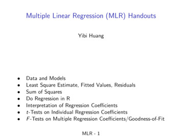
3Logistic RegressionRelated procedures. Use the Scatterplot procedure to screen your data for multicollinearity. Ifassumptions of multivariate normality and equal variance-covariance matrices are met, you maybe able to get a quicker solution using the Discriminant Analysis procedure. If all of your predictorvariables are categorical, you can also use the Loglinear procedure. If your dependent variableis continuous, use the Linear Regression procedure. You can use the ROC Curve procedure toplot probabilities saved with the Logistic Regression procedure.Obtaining a Logistic Regression AnalysisE From the menus choose:AnalyzeRegressionBinary Logistic.Figure 2-1Logistic Regression dialog boxE Select one dichotomous dependent variable. This variable may be numeric or string.E Select one or more covariates. To include interaction terms, select all of the variables involved inthe interaction and then select a*b .To enter variables in groups (blocks), select the covariates for a block, and click Next to specify anew block. Repeat until all blocks have been specified.Optionally, you can select cases for analysis. Choose a selection variable, and click Rule.

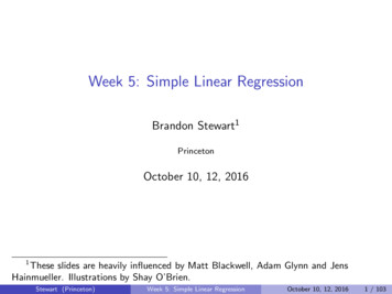
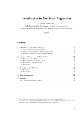
4Chapter 2Logistic Regression Set RuleFigure 2-2Logistic Regression Set Rule dialog boxCases defined by the selection rule are included in model estimation. For example, if you selecteda variable and equals and specified a value of 5, then only the cases for which the selected variablehas a value equal to 5 are included in estimating the model.Statistics and classification results are generated for both selected and unselected cases.This provides a mechanism for classifying new cases based on previously existing data, or forpartitioning your data into training and testing subsets, to perform validation on the modelgenerated.Logistic Regression Variable Selection MethodsMethod selection allows you to specify how independent variables are entered into the analysis.Using different methods, you can construct a variety of regression models from the same set ofvariables. Enter. A procedure for variable selection in which all variables in a block are entered in asingle step. Forward Selection (Conditional). Stepwise selection method with entry testing based onthe significance of the score statistic, and removal testing based on the probability of alikelihood-ratio statistic based on conditional parameter estimates. Forward Selection (Likelihood Ratio). Stepwise selection method with entry testing basedon the significance of the score statistic, and removal testing based on the probability of alikelihood-ratio statistic based on the maximum partial likelihood estimates. Forward Selection (Wald). Stepwise selection method with entry testing based on thesignificance of the score statistic, and removal testing based on the probability of the Waldstatistic. Backward Elimination (Conditional). Backward stepwise selection. Removal testing is based onthe probability of the likelihood-ratio statistic based on conditional parameter estimates. Backward Elimination (Likelihood Ratio). Backward stepwise selection. Removal testingis based on the probability of the likelihood-ratio statistic based on the maximum partiallikelihood estimates. Backward Elimination (Wald). Backward stepwise selection. Removal testing is based on theprobability of the Wald statistic.

5Logistic RegressionThe significance values in your output are based on fitting a single model. Therefore, thesignificance values are generally invalid when a stepwise method is used.All independent variables selected are added to a single regression model. However, you canspecify different entry methods for different subsets of variables. For example, you can enter oneblock of variables into the regression model using stepwise selection and a second block usingforward selection. To add a second block of variables to the regression model, click Next.Logistic Regression Define Categorical VariablesFigure 2-3Logistic Regression Define Categorical Variables dialog boxYou can specify details of how the Logistic Regression procedure will handle categorical variables:Covariates. Contains a list of all of the covariates specified in the main dialog box, either bythemselves or as part of an interaction, in any layer. If some of these are string variables or arecategorical, you can use them only as categorical covariates.Categorical Covariates. Lists variables identified as categorical. Each variable includes a notationin parentheses indicating the contrast coding to be used. String variables (denoted by the symbol following their names) are already present in the Categorical Covariates list. Select any othercategorical covariates from the Covariates list and move them into the Categorical Covariates list.Change Contrast. Allows you to change the contrast method. Available contrast methods are: Indicator. Contrasts indicate the presence or absence of category membership. The referencecategory is represented in the contrast matrix as a row of zeros. Simple. Each category of the predictor variable (except the reference category) is comparedto the reference category. Difference. Each category of the predictor variable except the first category is compared to theaverage effect of previous categories. Also known as reverse Helmert contrasts. Helmert. Each category of the predictor variable except the last category is compared tothe average effect of subsequent categories. Repeated. Each category of the predictor variable except the first category is compared to thecategory that precedes it.

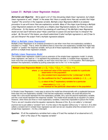
6Chapter 2 Polynomial. Orthogonal polynomial contrasts. Categories are assumed to be equally spaced.Polynomial contrasts are available for numeric variables only. Deviation. Each category of the predictor variable except the reference category is comparedto the overall effect.If you select Deviation, Simple, or Indicator, select either First or Last as the reference category.Note that the method is not actually changed until you click Change.String covariates must be categorical covariates. To remove a string variable from theCategorical Covariates list, you must remove all terms containing the variable from the Covariateslist in the main dialog box.Logistic Regression Save New VariablesFigure 2-4Logistic Regression Save New Variables dialog boxYou can save results of the logistic regression as new variables in the active dataset:Predicted Values. Saves values predicted by the model. Available options are Probabilities andGroup membership. Probabilities. For each case, saves the predicted probability of occurrence of the event. A tablein the output displays name and contents of any new variables. Predicted Group Membership. The group with the largest posterior probability, based ondiscriminant scores. The group the model predicts the case belongs to.Influence. Saves values from statistics that measure the influence of cases on predicted values.Available options are Cook’s, Leverage values, and DfBeta(s). Cook’s. The logistic regression analog of Cook’s influence statistic. A measure of how muchthe residuals of all cases would change if a particular case were excluded from the calculationof the regression coefficients.

7Logistic Regression Leverage Value. The relative influence of each observation on the model’s fit. DfBeta(s). The difference in beta value is the change in the regression coefficient that resultsfrom the exclusion of a particular case. A value is computed for each term in the model,including the constant.Residuals. Saves residuals. Available options are Unstandardized, Logit, Studentized,Standardized, and Deviance. Unstandardized Residuals. The difference between an observed value and the value predictedby the model. Logit Residual. The residual for the case if it is predicted in the logit scale. The logit residual isthe residual divided by the predicted probability times 1 minus the predicted probability. Studentized Residual. The change in the model deviance if a case is excluded. Standardized Residuals. The residual divided by an estimate of its standard deviation.Standardized residuals, which are also known as Pearson residuals, have a mean of 0 anda standard deviation of 1. Deviance. Residuals based on the model deviance.Export model information to XML file. Parameter estimates and (optionally) their covariances areexported to the specified file in XML (PMML) format. SmartScore and PASW Statistics Server(a separate product) can use this model file to apply the model information to other data filesfor scoring purposes.Logistic Regression OptionsFigure 2-5Logistic Regression Options dialog box

8Chapter 2You can specify options for your logistic regression analysis:Statistics and Plots. Allows you to request statistics and plots. Available options are Classificationplots, Hosmer-Lemeshow goodness-of-fit, Casewise listing of residuals, Correlations of estimates,Iteration history, and CI for exp(B). Select one of the alternatives in the Display group to displaystatistics and plots either At each step or, only for the final model, At last step. Hosmer-Lemeshow goodness-of-fit statistic. This goodness-of-fit statistic is more robust thanthe traditional goodness-of-fit statistic used in logistic regression, particularly for models withcontinuous covariates and studies with small sample sizes. It is based on grouping casesinto deciles of risk and comparing the observed probability with the expected probabilitywithin each decile.Probability for Stepwise. Allows you to control the criteria by which variables are entered into andremoved from the equation. You can specify criteria for Entry or Removal of variables. Probability for Stepwise. A variable is entered into the model if the probability of its scorestatistic is less than the Entry value and is removed if the probability is greater than theRemoval value. To override the default settings, enter positive values for Entry and Removal.Entry must be less than Removal.Classification cutoff. Allows you to determine the cut point for classifying cases. Cases withpredicted values that exceed the classification cutoff are classified as positive, while those withpredicted values smaller than the cutoff are classified as negative. To change the default, enter avalue between 0.01 and 0.99.Maximum Iterations. Allows you to change the maximum number of times that the model iteratesbefore terminating.Include constant in model. Allows you to indicate whether the model should include a constantterm. If disabled, the constant term will equal 0.LOGISTIC REGRESSION Command Additional FeaturesThe command syntax language also allows you to: Identify casewise output by the values or variable labels of a variable. Control the spacing of iteration reports. Rather than printing parameter estimates after everyiteration, you can request parameter estimates after every nth iteration. Change the criteria for terminating iteration and checking for redundancy. Specify a variable list for casewise listings. Conserve memory by holding the data for each split file group in an external scratch fileduring processing.See the Command Syntax Reference for complete syntax information.

ChapterMultinomial Logistic Regression3Multinomial Logistic Regression is useful for situations in which you want to be able to classifysubjects based on values of a set of predictor variables. This type of regression is similar to logisticregression, but it is more general because the dependent variable is not restricted to two categories.Example. In order to market films more effectively, movie studios want to predict what type offilm a moviegoer is likely to see. By performing a Multinomial Logistic Regression, the studiocan determine the strength of influence a person’s age, gender, and dating status has upon the typeof film they prefer. The studio can then slant the advertising campaign of a particular movietoward a group of people likely to go see it.Statistics. Iteration history, parameter coefficients, asymptotic covariance and correlation matrices,likelihood-ratio tests for model and partial effects, –2 log-likelihood. Pearson and deviancechi-square goodness of fit. Cox and Snell, Nagelkerke, and McFadden R2. Classification:observed versus predicted frequencies by response category. Crosstabulation: observed andpredicted frequencies (with residuals) and proportions by covariate pattern and response category.Methods. A multinomial logit model is fit for the full factorial model or a user-specified model.Parameter estimation is performed through an iterative maximum-likelihood algorithm.Data. The dependent variable should be categorical. Independent variables can be factors orcovariates. In general, factors should be categorical variables and covariates should be continuousvariables.Assumptions. It is assumed that the odds ratio of any two categories are independent of all otherresponse categories. For example, if a new product is introduced to a market, this assumptionstates that the market shares of all other products are affected proportionally equally. Also, given acovariate pattern, the responses are assumed to be independent multinomial variables.Obtaining a Multinomial Logistic RegressionE From the menus choose:AnalyzeRegressionMultinomial Logistic.9

10Chapter 3Figure 3-1Multinomial Logistic Regression dialog boxE Select one dependent variable.E Factors are optional and can be either numeric or categorical.E Covariates are optional but must be numeric if specified.

11Multinomial Logistic RegressionMultinomial Logistic RegressionFigure 3-2Multinomial Logistic Regression Model dialog boxBy default, the Multinomial Logistic Regression procedure produces a model with the factor andcovariate main effects, but you can specify a custom model or request stepwise model selectionwith this dialog box.Specify Model. A main-effects model contains the covariate and factor main effects but nointeraction effects. A full factorial model contains all main effects and all factor-by-factorinteractions. It does not contain covariate interactions. You can create a custom model to specifysubsets of factor interactions or covariate interactions, or request stepwise selection of modelterms.Factors & Covariates. The factors and covariates are listed.Forced Entry Terms. Terms added to the forced entry list are always included in the model.Stepwise Terms. Terms added to the stepwise list are included in the model according to one of thefollowing user-selected Stepwise Methods: Forward entry. This method begins with no stepwise terms in the model. At each step, the mostsignificant term is added to the model until none of the stepwise terms left out of the modelwould have a statistically significant contribution if added to the model.

12Chapter 3 Backward elimination. This method begins by entering all terms specified on the stepwise listinto the model. At each step, the least significant stepwise term is removed from the modeluntil all of the remaining stepwise terms have a statistically significant contribution to themodel. Forward stepwise. This method begins with the model that would be selected by the forwardentry method. From there, the algorithm alternates between backward elimination on thestepwise terms in the model and forward entry on the terms left out of the model. Thiscontinues until no terms meet the entry or removal criteria. Backward stepwise. This method begins with the model that would be selected by thebackward elimination method. From there, the algorithm alternates between forward entry onthe terms left out of the model an

The SPSS Statistics Statistical Procedures Companion, by Marija Norušis, has been published by Prentice Hall. A new version of this book, updated for PASW Statistics 18, is planned. The SPSS Statistics Advanced Statistical Procedures Companion, also based on PASW Statistics 18, is forthcoming.