Transcription
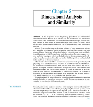
Chapter 5Dimensional Analysisand SimilarityMotivation. In this chapter we discuss the planning, presentation, and interpretationof experimental data. We shall try to convince you that such data are best presented indimensionless form. Experiments which might result in tables of output, or even multiple volumes of tables, might be reduced to a single set of curves—or even a singlecurve—when suitably nondimensionalized. The technique for doing this is dimensionalanalysis.Chapter 3 presented gross control-volume balances of mass, momentum, and energy which led to estimates of global parameters: mass flow, force, torque, total heattransfer. Chapter 4 presented infinitesimal balances which led to the basic partial differential equations of fluid flow and some particular solutions. These two chapters covered analytical techniques, which are limited to fairly simple geometries and welldefined boundary conditions. Probably one-third of fluid-flow problems can be attackedin this analytical or theoretical manner.The other two-thirds of all fluid problems are too complex, both geometrically andphysically, to be solved analytically. They must be tested by experiment. Their behavior is reported as experimental data. Such data are much more useful if they are expressed in compact, economic form. Graphs are especially useful, since tabulated datacannot be absorbed, nor can the trends and rates of change be observed, by most engineering eyes. These are the motivations for dimensional analysis. The technique istraditional in fluid mechanics and is useful in all engineering and physical sciences,with notable uses also seen in the biological and social sciences.Dimensional analysis can also be useful in theories, as a compact way to present ananalytical solution or output from a computer model. Here we concentrate on the presentation of experimental fluid-mechanics data.5.1 IntroductionBasically, dimensional analysis is a method for reducing the number and complexityof experimental variables which affect a given physical phenomenon, by using a sortof compacting technique. If a phenomenon depends upon n dimensional variables, dimensional analysis will reduce the problem to only k dimensionless variables, wherethe reduction n k 1, 2, 3, or 4, depending upon the problem complexity. Generally n k equals the number of different dimensions (sometimes called basic or pri277
278Chapter 5 Dimensional Analysis and Similaritymary or fundamental dimensions) which govern the problem. In fluid mechanics, thefour basic dimensions are usually taken to be mass M, length L, time T, and temperature , or an MLT system for short. Sometimes one uses an FLT system, with forceF replacing mass.Although its purpose is to reduce variables and group them in dimensionless form,dimensional analysis has several side benefits. The first is enormous savings in timeand money. Suppose one knew that the force F on a particular body immersed in astream of fluid depended only on the body length L, stream velocity V, fluid density , and fluid viscosity , that is,F f(L, V, , )(5.1)Suppose further that the geometry and flow conditions are so complicated that our integral theories (Chap. 3) and differential equations (Chap. 4) fail to yield the solutionfor the force. Then we must find the function f(L, V, , ) experimentally.Generally speaking, it takes about 10 experimental points to define a curve. To findthe effect of body length in Eq. (5.1), we have to run the experiment for 10 lengths L.For each L we need 10 values of V, 10 values of , and 10 values of , making a grandtotal of 104, or 10,000, experiments. At 50 per experiment—well, you see what weare getting into. However, with dimensional analysis, we can immediately reduceEq. (5.1) to the equivalent formF VL 2 2 g V L or(5.2)CF g(Re)i.e., the dimensionless force coefficient F/( V2L2) is a function only of the dimensionless Reynolds number VL/ . We shall learn exactly how to make this reduction inSecs. 5.2 and 5.3.The function g is different mathematically from the original function f, but it contains all the same information. Nothing is lost in a dimensional analysis. And think ofthe savings: We can establish g by running the experiment for only 10 values of thesingle variable called the Reynolds number. We do not have to vary L, V, , or separately but only the grouping VL/ . This we do merely by varying velocity V in, say,a wind tunnel or drop test or water channel, and there is no need to build 10 differentbodies or find 100 different fluids with 10 densities and 10 viscosities. The cost is nowabout 500, maybe less.A second side benefit of dimensional analysis is that it helps our thinking and planning for an experiment or theory. It suggests dimensionless ways of writing equationsbefore we waste money on computer time to find solutions. It suggests variables whichcan be discarded; sometimes dimensional analysis will immediately reject variables,and at other times it groups them off to the side, where a few simple tests will showthem to be unimportant. Finally, dimensional analysis will often give a great deal ofinsight into the form of the physical relationship we are trying to study.A third benefit is that dimensional analysis provides scaling laws which can convert data from a cheap, small model to design information for an expensive, large prototype. We do not build a million-dollar airplane and see whether it has enough liftforce. We measure the lift on a small model and use a scaling law to predict the lift on
5.1 Introduction279the full-scale prototype airplane. There are rules we shall explain for finding scalinglaws. When the scaling law is valid, we say that a condition of similarity exists between the model and the prototype. In the simple case of Eq. (5.1), similarity is achievedif the Reynolds number is the same for the model and prototype because the functiong then requires the force coefficient to be the same also:IfRem Repthen CFm CFp(5.3)where subscripts m and p mean model and prototype, respectively. From the definitionof force coefficient, this means thatFp p Vp Fm m VmLp Lm 22(5.4)for data taken where pVp Lp / p mVm Lm / m. Equation (5.4) is a scaling law: If youmeasure the model force at the model Reynolds number, the prototype force at thesame Reynolds number equals the model force times the density ratio times the velocity ratio squared times the length ratio squared. We shall give more examples later.Do you understand these introductory explanations? Be careful; learning dimensionalanalysis is like learning to play tennis: There are levels of the game. We can establish someground rules and do some fairly good work in this brief chapter, but dimensional analysis in the broad view has many subtleties and nuances which only time and practice andmaturity enable you to master. Although dimensional analysis has a firm physical andmathematical foundation, considerable art and skill are needed to use it effectively.EXAMPLE 5.1A copepod is a water crustacean approximately 1 mm in diameter. We want to know the dragforce on the copepod when it moves slowly in fresh water. A scale model 100 times larger ismade and tested in glycerin at V 30 cm/s. The measured drag on the model is 1.3 N. For similar conditions, what are the velocity and drag of the actual copepod in water? Assume thatEq. (5.1) applies and the temperature is 20 C.SolutionFrom Table A.3 the fluid properties are:Water (prototype): p 0.001 kg/(m s) p 998 kg/m3Glycerin (model): m 1.5 kg/(m s) m 1263 kg/m3The length scales are Lm 100 mm and Lp 1 mm. We are given enough model data to compute the Reynolds number and force coefficient(1263 kg/m3)(0.3 m/s)(0.1 m) mVmLm 25.3Rem 1.5 kg/(m s) m1.3 NFm 1.14CFm (1263 kg/m3)(0.3 m/s)2(0.1 m)2 mVm2Lm2Both these numbers are dimensionless, as you can check. For conditions of similarity, the prototype Reynolds number must be the same, and Eq. (5.2) then requires the prototype force coefficient to be the same
280Chapter 5 Dimensional Analysis and Similarity998Vp(0.001)Rep Rem 25.3 0.001orVp 0.0253 m/s 2.53 cm/sAns.FpCFp CFm 1.14 998(0.0253)2(0.001)2orFp 7.3110 7 NAns.It would obviously be difficult to measure such a tiny drag force.Historically, the first person to write extensively about units and dimensional reasoningin physical relations was Euler in 1765. Euler’s ideas were far ahead of his time, as werethose of Joseph Fourier, whose 1822 book Analytical Theory of Heat outlined what is nowcalled the principle of dimensional homogeneity and even developed some similarity rulesfor heat flow. There were no further significant advances until Lord Rayleigh’s book in1877, Theory of Sound, which proposed a “method of dimensions” and gave several examples of dimensional analysis. The final breakthrough which established the method aswe know it today is generally credited to E. Buckingham in 1914 [29], whose paper outlined what is now called the Buckingham pi theorem for describing dimensionless parameters (see Sec. 5.3). However, it is now known that a Frenchman, A. Vaschy, in 1892 anda Russian, D. Riabouchinsky, in 1911 had independently published papers reporting results equivalent to the pi theorem. Following Buckingham’s paper, P. W. Bridgman published a classic book in 1922 [1], outlining the general theory of dimensional analysis. Thesubject continues to be controversial because there is so much art and subtlety in using dimensional analysis. Thus, since Bridgman there have been at least 24 books published onthe subject [2 to 25]. There will probably be more, but seeing the whole list might makesome fledgling authors think twice. Nor is dimensional analysis limited to fluid mechanics or even engineering. Specialized books have been written on the application of dimensional analysis to metrology [26], astrophysics [27], economics [28], building scalemodels [36], chemical processing pilot plants [37], social sciences [38], biomedical sciences [39], pharmacy [40], fractal geometry [41], and even the growth of plants [42].5.2 The Principle ofDimensional HomogeneityIn making the remarkable jump from the five-variable Eq. (5.1) to the two-variableEq. (5.2), we were exploiting a rule which is almost a self-evident axiom in physics.This rule, the principle of dimensional homogeneity (PDH), can be stated as follows:If an equation truly expresses a proper relationship between variables in a physicalprocess, it will be dimensionally homogeneous; i.e., each of its additive terms willhave the same dimensions.All the equations which are derived from the theory of mechanics are of this form. Forexample, consider the relation which expresses the displacement of a falling bodyS S0V0t 1 2gt2(5.5)Each term in this equation is a displacement, or length, and has dimensions {L}. Theequation is dimensionally homogeneous. Note also that any consistent set of units canbe used to calculate a result.
5.2 The Principle of Dimensional Homogeneity281Consider Bernoulli’s equation for incompressible flowp 1 V22gz const(5.6)Each term, including the constant, has dimensions of velocity squared, or {L2T 2}.The equation is dimensionally homogeneous and gives proper results for any consistent set of units.Students count on dimensional homogeneity and use it to check themselves whenthey cannot quite remember an equation during an exam. For example, which is it:S 12 gt2?S 12 g2t?or(5.7)By checking the dimensions, we reject the second form and back up our faulty memory. We are exploiting the principle of dimensional homogeneity, and this chapter simply exploits it further.Equations (5.5) and (5.6) also illustrate some other factors that often enter into a dimensional analysis:Dimensional variables are the quantities which actually vary during a given caseand would be plotted against each other to show the data. In Eq. (5.5), they areS and t; in Eq. (5.6) they are p, V, and z. All have dimensions, and all can benondimensionalized as a dimensional-analysis technique.Dimensional constants may vary from case to case but are held constant during agiven run. In Eq. (5.5) they are S0, V0, and g, and in Eq. (5.6) they are , g,and C. They all have dimensions and conceivably could be nondimensionalized, but they are normally used to help nondimensionalize the variables in theproblem.Pure constants have no dimensions and never did. They arise from mathematicalmanipulations. In both Eqs. (5.5) and (5.6) they are 12 and the exponent 2, bothof which came from an integration: t dt 12 t2, V dV 12 V2. Other commondimensionless constants are and e.Note that integration and differentiation of an equation may change the dimensionsbut not the homogeneity of the equation. For example, integrate or differentiateEq. (5.5): S dt S t0V0t2 1 2dS V0dtgtgt3 1 6(5.8a)(5.8b)In the integrated form (5.8a) every term has dimensions of {LT}, while in the derivative form (5.8b) every term is a velocity {LT 1}.Finally, there are some physical variables that are naturally dimensionless by virtueof their definition as ratios of dimensional quantities. Some examples are strain (changein length per unit length), Poisson’s ratio (ratio of transverse strain to longitudinal strain),and specific gravity (ratio of density to standard water density). All angles are dimensionless (ratio of arc length to radius) and should be taken in radians for this reason.The motive behind dimensional analysis is that any dimensionally homogeneousequation can be written in an entirely equivalent nondimensional form which is more
282Chapter 5 Dimensional Analysis and Similaritycompact. Usually there is more than one method of presenting one’s dimensionless dataor theory. Let us illustrate these concepts more thoroughly by using the falling-bodyrelation (5.5) as an example.Ambiguity: The Choice ofVariables and Scaling Parameters1Equation (5.5) is familiar and simple, yet illustrates most of the concepts of dimensional analysis. It contains five terms (S, S0, V0, t, g) which we may divide, in our thinking, into variables and parameters. The variables are the things which we wish to plot,the basic output of the experiment or theory: in this case, S versus t. The parametersare those quantities whose effect upon the variables we wish to know: in this case S0,V0, and g. Almost any engineering study can be subdivided in this manner.To nondimensionalize our results, we need to know how many dimensions are contained among our variables and parameters: in this case, only two, length {L} and time{T}. Check each term to verify this:{S} {S0} {L}{t} {T}{V0} {LT 1}{g} {LT 2}Among our parameters, we therefore select two to be scaling parameters, used to define dimensionless variables. What remains will be the “basic” parameter(s) whose effect we wish to show in our plot. These choices will not affect the content of our data,only the form of their presentation. Clearly there is ambiguity in these choices, something that often vexes the beginning experimenter. But the ambiguity is deliberate. Itspurpose is to show a particular effect, and the choice is yours to make.For the falling-body problem, we select any two of the three parameters to be scaling parameters. Thus we have three options. Let us discuss and display them in turn.Option 1: Scaling parameters S0 and V0: the effect of gravity g.First use the scaling parameters (S0, V0) to define dimensionless (*) displacementand time. There is only one suitable definition for each:2SS* S0Vtt* 0 S0(5.9)Substitute these variables into Eq. (5.5) and clean everything up until each term is dimensionless. The result is our first option:S* 1t*1 t*22gS0 V 02(5.10)This result is shown plotted in Fig. 5.1a. There is a single dimensionless parameter ,which shows here the effect of gravity. It cannot show the direct effects of S0 and V0,since these two are hidden in the ordinate and abscissa. We see that gravity increasesthe parabolic rate of fall for t* 0, but not the initial slope at t* 0. We would learnthe same from falling-body data, and the plot, within experimental accuracy, wouldlook like Fig. 5.1a.1I am indebted to Prof. Jacques Lewalle of Syracuse University for suggesting, outlining, and clarifying this entire discussion.2Make them proportional to S and t. Do not define dimensionless terms upside down: S0/S or S0/(V0t).The plots will look funny, users of your data will be confused, and your supervisor will be angry. It is nota good idea.
5.2 The Principle of Dimensional Homogeneity58g S0 2V0210.5gSV020g S0 2V0216S ** SS00.50.2S * 4328304221032001Vtt* 0S02gtt ** V0(a)(b)13108V0S *** SS0 gS0Fig. 5.1 Three entirely equivalentdimensionless presentations of thefalling-body problem, Eq. (5.5): theeffect of (a) gravity, (b) initial displacement, and (c) initial velocity.All plots contain the same information. 2160.504200123t *** t g / S0(c)Option 2: Scaling parameters V0 and g: the effect of initial displacement S0.Now use the new scaling parameters (V0, g) to define dimensionless (**) displacement and time. Again there is only one suitable definition:SgS** 2 V0gt** t V0(5.11)Substitute these variables into Eq. (5.5) and clean everything up again. The result isour second option:1gS0S** t** t**2 (5.12)2V 02
284Chapter 5 Dimensional Analysis and SimilarityThis result is plotted in Fig. 5.1b. The same single parameter again appears and hereshows the effect of initial displacement, which merely moves the curves upward without changing their shape.Option 3: Scaling parameters S0 and g: the effect of initial speed V0.Finally use the scaling parameters (S0, g) to define dimensionless (***) displacement and time. Again there is only one suitable definition:SS*** S0 gt*** t S01/2(5.13)Substitute these variables into Eq. (5.5) and clean everything up as usual. The resultis our third and final option:S*** 1 t***1 t***221V0 g S 0(5.14)This final presentation is shown in Fig. 5.1c. Once again the parameter appears, butwe have redefined it upside down, 1/ , so that our display parameter V0 is inthe numerator and is linear. This is our free choice and simply improves the display.Figure 5.1c shows that initial velocity increases the falling displacement and that theincrease is proportional to time.Note that, in all three options, the same parameter appears but has a differentmeaning: dimensionless gravity, initial displacement, and initial velocity. The graphs,which contain exactly the same information, change their appearance to reflect thesedifferences.Whereas the original problem, Eq. (5.5), involved five quantities, the dimensionlesspresentations involve only three, having the formS fcn(t , )gS0 V 02(5.15)The reduction 5 3 2 should equal the number of fundamental dimensions involvedin the problem {L, T}. This idea led to the pi theorem (Sec. 5.3).The choice of scaling variables is left to the user, and the resulting dimensionlessparameters have differing interpretations. For example, in the dimensionless drag-forceformulation, Eq. (5.2), it is now clear that the scaling parameters were , V, and L,since they appear in both the drag coefficient and the Reynolds number. Equation (5.2)can thus be interpreted as the variation of dimensionless force with dimensionless viscosity, with the scaling-parameter effects mixed between CF and Re and therefore notimmediately evident.Suppose that we wish to study drag force versus velocity. Then we would not useV as a scaling parameter. We would use ( , , L) instead, and the final dimensionlessfunction would become FCF fcn(Re) 2 VLRe (5.16)In plotting these data, we would not be able to discern the effect of or , since theyappear in both dimensionless groups. The grouping CF again would mean dimension-
5.2 The Principle of Dimensional Homogeneity285less force, and Re is now interpreted as either dimensionless velocity or size.3 The plotwould be quite different compared to Eq. (5.2), although it contains exactly the sameinformation. The development of parameters such as CF and Re from the initial variables is the subject of the pi theorem (Sec. 5.3).Some Peculiar EngineeringEquationsThe foundation of the dimensional-analysis method rests on two assumptions: (1) Theproposed physical relation is dimensionally homogeneous, and (2) all the relevant variables have been included in the proposed relation.If a relevant variable is missing, dimensional analysis will fail, giving either algebraic difficulties or, worse, yielding a dimensionless formulation which does not resolve the process. A typical case is Manning’s open-channel formula, discussed in Example 1.4:1.49V R2/3S1/2(1)nSince V is velocity, R is a radius, and n and S are dimensionless, the formula is not dimensionally homogeneous. This should be a warning that (1) the formula changes if theunits of V and R change and (2) if valid, it represents a very special case. Equation (1)in Example 1.4 (see above) predates the dimensional-analysis technique and is validonly for water in rough channels at moderate velocities and large radii in BG units.Such dimensionally inhomogeneous formulas abound in the hydraulics literature.Another example is the Hazen-Williams formula [30] for volume flow of water througha straight smooth pipedp 0.54Q 61.9D2.63 (5.17)dx where D is diameter and dp/dx is the pressure gradient. Some of these formulas arisebecause numbers have been inserted for fluid properties and other physical data intoperfectly legitimate homogeneous formulas. We shall not give the units of Eq. (5.17)to avoid encouraging its use.On the other hand, some formulas are “constructs” which cannot be made dimensionally homogeneous. The “variables” they relate cannot be analyzed by the dimensional-analysis technique. Most of these formulas are raw empiricisms convenient to asmall group of specialists. Here are three examples:25,000B 100 R(5.18)140S 130 API(5.19)3.741720.0147DE 0.26tR DEtR(5.20)Equation (5.18) relates the Brinell hardness B of a metal to its Rockwell hardness R.Equation (5.19) relates the specific gravity S of an oil to its density in degrees API.3We were lucky to achieve a size effect because in this case L, a scaling parameter, did not appear inthe drag coefficient.
286Chapter 5 Dimensional Analysis and SimilarityEquation (5.20) relates the viscosity of a liquid in DE, or degrees Engler, to its viscosity tR in Saybolt seconds. Such formulas have a certain usefulness when communicated between fellow specialists, but we cannot handle them here. Variables likeBrinell hardness and Saybolt viscosity are not suited to an MLT dimensional system.5.3 The Pi TheoremThere are several methods of reducing a number of dimensional variables into a smallernumber of dimensionless groups. The scheme given here was proposed in 1914 byBuckingham [29] and is now called the Buckingham pi theorem. The name pi comesfrom the mathematical notation , meaning a product of variables. The dimensionlessgroups found from the theorem are power products denoted by 1, 2, 3, etc. Themethod allows the pis to be found in sequential order without resorting to free exponents.The first part of the pi theorem explains what reduction in variables to expect:If a physical process satisfies the PDH and involves n dimensional variables, it canbe reduced to a relation between only k dimensionless variables or ’s. The reduction j n k equals the maximum number of variables which do not form a piamong themselves and is always less than or equal to the number of dimensions describing the variables.Take the specific case of force on an immersed body: Eq. (5.1) contains five variablesF, L, U, , and described by three dimensions {MLT}. Thus n 5 and j 3. Therefore it is a good guess that we can reduce the problem to k pis, with k n j 5 3 2. And this is exactly what we obtained: two dimensionless variables 1 CF and 2 Re. On rare occasions it may take more pis than this minimum (see Example5.5).The second part of the theorem shows how to find the pis one at a time:Find the reduction j, then select j scaling variables which do not form a pi amongthemselves.4 Each desired pi group will be a power product of these j variables plusone additional variable which is assigned any convenient nonzero exponent. Eachpi group thus found is independent.To be specific, suppose that the process involves five variables 1 f( 2, 3, 4, 5)Suppose that there are three dimensions {MLT} and we search around and find that indeed j 3. Then k 5 3 2 and we expect, from the theorem, two and only twopi groups. Pick out three convenient variables which do not form a pi, and supposethese turn out to be 2, 3, and 4. Then the two pi groups are formed by power products of these three plus one additional variable, either 1 or 5: 1 ( 2)a( 3)b( 4)c 1 M0L0T0 2 ( 2)a( 3)b( 4)c 5 M0L0T0Here we have arbitrarily chosen 1 and 5, the added variables, to have unit exponents.Equating exponents of the various dimensions is guaranteed by the theorem to giveunique values of a, b, and c for each pi. And they are independent because only 14Make a clever choice here because all pis will contain these j variables in various groupings.
5.3 The Pi TheoremTable 5.1 Dimensions of FluidMechanics ocityAccelerationSpeed of soundVolume flowMass flowPressure, stressStrain rateAngleAngular velocityViscosityKinematic viscositySurface tensionForceMoment, torquePowerWork, energyDensityTemperatureSpecific heatSpecific weightThermal conductivityExpansion coefficientSymbolLA VdV/dtaQṁp, FMPW, E Tcp, c k MLT LL2L3LT 1LT 2LT 1L3T 1MT 1ML 1T 2T 1NoneT 1ML 1T 1L2T 1MT 2MLT 2ML2T 2ML2T –3ML2T 2ML–3 L2T 2 1ML–2T 2MLT –3 1 1FLT LL2L3LT 1LT 2LT 1L3T 1FTL 1FL 2T 1NoneT 1FTL 2L2T 1FL 1FFLFLT 1FLFT2L–4 L2T 2 1FL 3FT 1 1 1contains 1 and only 2 contains 5. It is a very neat system once you get used to theprocedure. We shall illustrate it with several examples.Typically, six steps are involved:1.2.3.4.5.List and count the n variables involved in the problem. If any important variables are missing, dimensional analysis will fail.List the dimensions of each variable according to {MLT } or {FLT }. A list isgiven in Table 5.1.Find j. Initially guess j equal to the number of different dimensions present, andlook for j variables which do not form a pi product. If no luck, reduce j by 1and look again. With practice, you will find j rapidly.Select j scaling parameters which do not form a pi product. Make sure theyplease you and have some generality if possible, because they will then appearin every one of your pi groups. Pick density or velocity or length. Do not picksurface tension, e.g., or you will form six different independent Weber-numberparameters and thoroughly annoy your colleagues.Add one additional variable to your j repeating variables, and form a powerproduct. Algebraically find the exponents which make the product dimensionless. Try to arrange for your output or dependent variables (force, pressure drop,torque, power) to appear in the numerator, and your plots will look better. Do
288Chapter 5 Dimensional Analysis and Similarity6.this sequentially, adding one new variable each time, and you will find alln j k desired pi products.Write the final dimensionless function, and check your work to make sure all pigroups are dimensionless.EXAMPLE 5.2Repeat the development of Eq. (5.2) from Eq. (5.1), using the pi theorem.SolutionStep 1Write the function and count variables:F f(L, U, , ) there are five variables (n 5)Step 2List dimensions of each variable. From Table 5.1F{MLTL 2} U{L}{LT 1 3} 1 1{ML }{ML T}Step 3Find j. No variable contains the dimension , and so j is less than or equal to 3 (MLT). We inspect the list and see that L, U, and cannot form a pi group because only contains mass andonly U contains time. Therefore j does equal 3, and n j 5 3 2 k. The pi theoremguarantees for this problem that there will be exactly two independent dimensionless groups.Step 4Select repeating j variables. The group L, U, we found in step 3 will do fine.Step 5Combine L, U, with one additional variable, in sequence, to find the two pi products.First add force to find 1. You may select any exponent on this additional term as you please,to place it in the numerator or denominator to any power. Since F is the output, or dependent,variable, we select it to appear to the first power in the numerator: 1 LaUb cF (L)a(LT 1)b(ML 3)c( MLT 2) M0L0T0Equate exponents:Length:ab 3c1 0c1 0Mass: bTime: 2 0We can solve explicitly fora 2b 2c 1ThereforeF 1 L 2U 2 1F 2 2 CF U LAns.This is exactly the right pi group as in Eq. (5.2). By varying the exponent on F, we could havefound other equivalent groups such as UL 1/2/F1/2.
5.3 The Pi Theorem289Finally, add viscosity to L, U, and to find 2. Select any power you like for viscosity. Byhindsight and custom, we select the power 1 to place it in the denominator: 2 LaUb c 1 La(LT 1)b(ML 3)c(ML 1T 1) 1 M0L0T0Equate exponents:Length:ab 3c1 0c 1 0Mass: bTime:1 0from which we finda b c 1 UL 2 L1U1 1 1 Re ThereforeAns.We know we are finished; this is the second and last pi group. The theorem guarantees that thefunctional relationship must be of the equivalent form ULF 2 2 g U L Ans.which is exactly Eq. (5.2).EXAMPLE 5.3Reduce the falling-body relationship, Eq. (5.5), to a function of dimensionless variables. Whyare there three different formulations?SolutionWrite the function and count variablesS f(t, S0, V0, g) five variables (n 5)List the dimensions of each variable, from Table 5.1:S{L}t{T}S0{L}V0LTg 1}{LT 2}There are only two primary dimensions
5.2 The Principle of Dimensional Homogeneity Re p Re m 25.3 998V 0. p 0 (0 0. 1 001) or V p 0.0253 m/s 2.53 cm/s Ans. C Fp C Fm 1.14 or F p 7.31 10 7 N Ans. It would obviously be difficult to measure such a tiny drag force. Historically, the first person to write extensively about units and dimensional reasoning