Transcription
MS Excel Exercise #4: Monthly BudgetIn this exercise you will be creating a Budget Spreadsheet that can be used to calculate your monthly and annualexpenses. This type of spreadsheet is a very valuable tool as it can not only be used to track expenses but can be used tohelp you get a better understanding of what it is going to cost you to live and whether or not your current income willsupport your needs and wants.1. Begin by opening up a new worksheet in Microsoft Excel.2. Copy the following spreadsheet exactly as show below. Use the same rows and columns as shown. Enter in thecategory headings and the amounts of money spent for each day in each category.3. In Column N, enter formulas that calculate the total annual (12 months) income and expenses for each category.4. In Row 31, enter formulas that calculate the total expense amounts for each Month. (Note that Row 4 is incomeand not an expense!!)5.In Row 32, enter formulas that calculate the amount of money saved each month. This would be determined bysubtracting your Monthly Expenses from your Monthly Income. Use Conditional Formatting to format theSavings cells so that if the number is a negative it is RED and in (PARENTHESIS). Example: ( 554.00) But, if thenumber is positive, it will appear BLACK and BOLD and without brackets.6. In Cell N34, Create a formula that will calculate your Annual Savings Balance. This would be determined bysubtracting your total annual income from your total annual expenses, and represents the amount of money
you have saved during the year OR the amount you are in DEBT!!! Add the same conditional formatting that youdid in step 5.7. All numbers in your spreadsheet should be considered to be CURRENCY and formatted to appear with dollarsigns ( ) and with two decimal places. Example: 1200.508. Save the workbook in your Excel folder as Review Ex. 4MS Excel Exercise #5: Travel ExpensesIn this lesson you will again be creating a spreadsheet that may look a bit more complex but actually uses simpleformulas and functions that you have already used in previous lessons.Assume that you are a member of the National Honor Society and the club just returned from a multi-day field trip. Youwere given a 600.00 budget to spend on transportation, motel expenses, food, and entertainment. Your club advisorasked for an accounting of your expenditures and for you to return any club money that you did not spend.1. Begin by opening up a new worksheet in Microsoft Excel.2. Copy the following spreadsheet exactly as show below. Use the same rows and columns as shown. Enter in thecategory headings and the amounts of money spent for each day in each category.SPECIFIC TASKS3. EXPENSES: All of the dollar amounts ( ) shown above are expenses. Make sure you have entered them into thecorrect cells. For all the cells that deal with expenses you will need to format the cells so that they show the symbol and two decimal places. (Example: 4.25) NOTE: Mileage is not currency so should not be formatted assuch.
4. FORMULAS: Create and enter the following formulas.Mileage Reimbursement: You get reimbursed 0.35 (35 cents) per mile driven. Calculate in Cells C5through F5 the amount you should be reimbursed for each day.Amount Spent / Category: Create formulas that calculate the total spent for all 4 days for each expensecategory and place these formulas in Column G, Cells G5 through G13.Daily Amount Spent: Create formulas that calculate the total spent for each individual day. Place theseformulas in Row 15, Cells C15 through F15.Expense Summaries: Create formulas that calculate the total amounts spent for all four days incombined categories of Transportation (Mileage expenses) Lodging (Motel Room) Food (Breakfast,Lunch & Dinner) and Entertainment (Admissions and Programs).Amount Returned: Create a formula that subtracts your total expenses for the entire trip from the 600.00 provided you to determine the amount of money you need to return to your advisor.5. Save the workbook in your Excel folder as Review Ex. 5MS Excel Exercise #6: Basketball StatisticsIn this lesson you will be creating a Spreadsheet that can be used to calculate statistics from a Armstrong Twp. HighSchool basketball game. This type of spreadsheet is a useful tool in helping to evaluate individual performances andtrack team trends in games throughout the season.1. Begin by opening up a new worksheet in Microsoft Excel.2. Copy the following spreadsheet exactly as show below. Make sure that you copy the exact statistics shown onthe table. Use the same rows and columns as shown.
3. For each Column, B through G, enter a formula that will ADD the total for Rows 5 through 16.4.In Column H, Rows 5 - 16, you will need to create a formula that will calculate the total number of points thateach player scored. This formula will need to have three parts. Use the following information for making yourformula.For each Field Goal Made the player scores 2 pointsFor each 3 Pointer Made the player scores 3 pointsFor each Free Throw Made the player scores 1 point5. In Cell H17, enter a formula that calculates the Total Number of Points score by the Team.6. In Column I, calculate the Percentage of the Total Team Points scored for each individual playerPercentage of Total Team Points Total Points (player) / Total Team PointsYou may want to use the Absolute Reference symbol ( ) in this formula ( Example: C 1 )7. Make sure that Column I displays the calculated numbers with a % sign.8.In Column J, calculate the Percentage of Field Goals Made by each player.% Made Number Made / Number AttemptedIN ADDITION.If a player did not attempt to shoot or did not score any points,your formulas for Column J (% Field Goals Made) must not display the error message #DIV/0!In order to prevent this, you must create an IF statement that will print NA (Not Applicable) for all players who did notattempt a shot or did not score any points.IF Number Attempted 0, then “NA”, else Number Made/Number Attempted9. In Column K, you will repeat this same kind of IF formula that you created in Column I.In Column K, calculate the Percentage of the 3 pointers Made by each Player% Made Number 3 Pointers Made / Number 3 Pointers AttemptedYou will need to incorporate this formula into an IF statement that will print NA (Not Applicable) for all playerswho did not attempt a three point shot or did not score any points. Remember! The cells must not display theerror message #DIV/0!10. Make sure that Column K displays the calculated numbers with a % sign.11. Column L, you will repeat this same kind of IF formula that you created in Column I.In Column L, calculate the Percentage of the Free Throws Made by each Player% Made Number Free Throws Made / Number AttemptedYou will need to incorporate this formula into an IF statement that will print NA (Not Applicable) for all playerswho did not attempt a free throw or did not score any points. Remember! The cells must not display the errormessage #DIV/0!
12. Make sure that Column K displays the calculated numbers with a % sign.13. In Cells J17, enter a formula that will calculate the overall Team 2 pt. Shooting %14. In Cells K17, enter a formula that will calculate the overall Team 3 pt. Shooting %15. In Cells L17, enter a formula that will calculate the overall Team Free Throw Shooting %16. Save the workbook in your Excel folder as Review Ex. 6MS Excel Exercise #7: Spreadsheet Functions & FormulasYour teacher, Ms. Schleef, has asked you to help her set up an Excel Spreadsheet that will organize the grades of herInformation Processing students. She has given you the following student records and would like for you to organize itinto grade book that can be used to calculate and record student test grades.1. Open a new worksheet in Microsoft Excel.2. Create an appropriate Title for the grade book worksheet and list your name as the author of it.3. The following information must be placed onto an organized on a spreadsheet. Use appropriate columnheadings.Student Last Names and their Scores for Test #1, #2, #3Aaronson: 78, 89, 80Ellenberg: 60, 70, 73Costello: 67, 79, 80Garcia: 84, 91, 76Kelly: 75, 90, 93Laney: 98, 86, 70Jae Woo: 72, 80, 70Hathaway: 87. 68, 80Mortenson: 66, 53, 71Diones: 88, 91, 80Barnett: 71, 77, 91Fallstaff: 76, 90, 904. Change the column widths so that the name column fits the widest entry.5. Enter formulas to calculate the following.a. Each Individual Student’s Combined Test Average.b. The Overall Class Average for each Test (Test #1, #2, & #3)6. Ms. Schleef wants to identify all students who have overall grades of less than 70%. Create an IF Function thatwill evaluate each students overall average test grade and will print out the words, "Study Hall" if their averageis below 70%7. Format all averages to one decimal place.8.Center all column headings and Bold them9. Sort the student in alphabetical order.10. Save the workbook in your Excel folder as Review Ex. 7
1. Begin by opening up a new worksheet in Microsoft Excel. 2. Copy the following spreadsheet exactly as show below. Use the same rows and columns as shown. Enter in the category headings and the amounts of money spent for each day in each category. SPECIFIC TASKS 3. EXPENSES: All of the dollar amounts ( ) shown above are expenses. Make sure you have entered them into the