Transcription
IEOR 269, Spring 2010Integer Programming and Combinatorial OptimizationProfessor Dorit S. HochbaumContents1 Introduction12 Formulation of some ILP2.1 0-1 knapsack problem . . . . . . . . . . . . . . . . . . . . . . . . . . . . . . . . . . .2.2 Assignment problem . . . . . . . . . . . . . . . . . . . . . . . . . . . . . . . . . . . .2223 Non-linear Objective functions3.1 Production problem with set-up costs3.2 Piecewise linear cost function . . . . .3.3 Piecewise linear convex cost function .3.4 Disjunctive constraints . . . . . . . . .44567problems. . . . . . . . . . . . . . . . . . . . . . . . . . . . . . . . . . . . . . . . . . . . . . . . . . . . . . . . . . . . . . . . . . . . . . . . . . . . . . . . . . . . . . . . . . . . . . . . .77774 Some famous combinatorial4.1 Max clique problem . . .4.2 SAT (satisfiability) . . . .4.3 Vertex cover problem . . .5 General optimization86 Neighborhood6.1 Exact neighborhood . . . . . . . . . . . . . . . . . . . . . . . . . . . . . . . . . . . .887 Complexity of algorithms7.1 Finding the maximum element7.2 0-1 knapsack . . . . . . . . . .7.3 Linear systems . . . . . . . . .7.4 Linear Programming . . . . . .99910118 Some interesting IP formulations128.1 The fixed cost plant location problem . . . . . . . . . . . . . . . . . . . . . . . . . . 128.2 Minimum/maximum spanning tree (MST) . . . . . . . . . . . . . . . . . . . . . . . . 129 The Minimum Spanning Tree (MST) Problemi13
IEOR269 notes, Prof. Hochbaum, 2010ii10 General Matching Problem1410.1 Maximum Matching Problem in Bipartite Graphs . . . . . . . . . . . . . . . . . . . . 1410.2 Maximum Matching Problem in Non-Bipartite Graphs . . . . . . . . . . . . . . . . . 1510.3 Constraint Matrix Analysis for Matching Problems . . . . . . . . . . . . . . . . . . . 1611 Traveling Salesperson Problem (TSP)1711.1 IP Formulation for TSP . . . . . . . . . . . . . . . . . . . . . . . . . . . . . . . . . . 1712 Discussion of LP-Formulation for MST1813 Branch-and-Bound2013.1 The Branch-and-Bound technique . . . . . . . . . . . . . . . . . . . . . . . . . . . . 2013.2 Other Branch-and-Bound techniques . . . . . . . . . . . . . . . . . . . . . . . . . . . 2214 Basic graph definitions2315 Complexity analysis15.1 Measuring quality of an algorithm . .15.1.1 Examples . . . . . . . . . . . .15.2 Growth of functions . . . . . . . . . .15.3 Definitions for asymptotic comparisons15.4 Properties of asymptotic notation . . .15.5 Caveats of complexity analysis . . . .24242426262627. . . . . . . . . . . . . . . . . . .of functions. . . . . . . . . . . . .16 Complexity classes and NP-completeness2816.1 Search vs. Decision . . . . . . . . . . . . . . . . . . . . . . . . . . . . . . . . . . . . . 2816.2 The class NP . . . . . . . . . . . . . . . . . . . . . . . . . . . . . . . . . . . . . . . . 2917 Addendum on Branch and Bound18 Complexity classes and NP-completeness18.1 Search vs. Decision . . . . . . . . . . . . .18.2 The class NP . . . . . . . . . . . . . . . .18.2.1 Some Problems in NP . . . . . . .18.3 The class co-NP . . . . . . . . . . . . . .18.3.1 Some Problems in co-NP . . . . .18.4 NPand co-NP . . . . . . . . . . . . . . . .18.5 NP-completeness and reductions . . . . .18.5.1 Reducibility . . . . . . . . . . . . .18.5.2 NP-Completeness . . . . . . . . . .19 The19.119.219.330.Chinese Checkerboard Problem and a First LookProblem Setup . . . . . . . . . . . . . . . . . . . . . . .The First Integer Programming Formulation . . . . . . .An Improved ILP Formulation . . . . . . . . . . . . . .at. . . .31313233343434353536Cutting Planes40. . . . . . . . . . . . . . 40. . . . . . . . . . . . . . 40. . . . . . . . . . . . . . 4020 Cutting Planes4320.1 Chinese checkers . . . . . . . . . . . . . . . . . . . . . . . . . . . . . . . . . . . . . . 4320.2 Branch and Cut . . . . . . . . . . . . . . . . . . . . . . . . . . . . . . . . . . . . . . . 44
IEOR269 notes, Prof. Hochbaum, 2010iii21 The geometry of Integer Programs and Linear Programs4521.1 Cutting planes for the Knapsack problem . . . . . . . . . . . . . . . . . . . . . . . . 4521.2 Cutting plane approach for the TSP . . . . . . . . . . . . . . . . . . . . . . . . . . . 4622 Gomory cuts4623 Generating a Feasible Solution for TSP4724 Diophantine Equations4824.1 Hermite Normal Form . . . . . . . . . . . . . . . . . . . . . . . . . . . . . . . . . . . 4925 Optimization with linear set of equality constraints5126 Balas’s additive algorithm5127 Held and Karp’s algorithm for TSP5428 Lagrangian Relaxation5529 Lagrangian Relaxation5930 Complexity of Nonlinear Optimization30.1 Input for a Polynomial Function . . . . . . . .30.2 Table Look-Up . . . . . . . . . . . . . . . . . .30.3 Examples of Non-linear Optimization Problems30.4 Impossibility of strongly polynomial algorithmsmization . . . . . . . . . . . . . . . . . . . . . . . . .for. . . . . . . . . . . . . . . . . . . . . . . . . . . . . . . . . . . . . . . . . . . .nonlinear (non-quadratic). . . . . . . . . . . . . . .61. . . . 61. . . . 61. . . . 62opti. . . . 6431 The General Network Flow Problem Setup6532 Shortest Path Problem6833 Maximum Flow Problem33.1 Setup . . . . . . . . . . . . . . . . . . . . . . . . . .33.2 Algorithms . . . . . . . . . . . . . . . . . . . . . . .33.2.1 Ford-Fulkerson algorithm . . . . . . . . . . .33.2.2 Capacity scaling algorithm . . . . . . . . . .33.3 Maximum-flow versus Minimum Cost Network Flow33.4 Formulation . . . . . . . . . . . . . . . . . . . . . . .6969717274757534 Minimum Cut Problem7734.1 Minimum s-t Cut Problem . . . . . . . . . . . . . . . . . . . . . . . . . . . . . . . . . 7734.2 Formulation . . . . . . . . . . . . . . . . . . . . . . . . . . . . . . . . . . . . . . . . . 7835 Selection Problem7936 A Production/Distribution Network: MCNF Formulation8136.1 Problem Description . . . . . . . . . . . . . . . . . . . . . . . . . . . . . . . . . . . . 8136.2 Formulation as a Minimum Cost Network Flow Problem . . . . . . . . . . . . . . . . 8336.3 The Optimal Solution to the Chairs Problem . . . . . . . . . . . . . . . . . . . . . . 84
IEOR269 notes, Prof. Hochbaum, 2010iv37 Transhipment Problem8738 Transportation Problem8738.1 Production/Inventory Problem as Transportation Problem . . . . . . . . . . . . . . . 8839 Assignment Problem40 Maximum Flow Problem40.1 A Package Delivery Problem9090. . . . . . . . . . . . . . . . . . . . . . . . . . . . . . . 9041 Shortest Path Problem9141.1 An Equipment Replacement Problem . . . . . . . . . . . . . . . . . . . . . . . . . . . 9242 Maximum Weight Matching9342.1 An Agent Scheduling Problem with Reassignment . . . . . . . . . . . . . . . . . . . 9343 MCNF Hierarchy9644 The maximum/minimum closure problem9644.1 A practical example: open-pit mining . . . . . . . . . . . . . . . . . . . . . . . . . . 9644.2 The maximum closure problem . . . . . . . . . . . . . . . . . . . . . . . . . . . . . . 9845 Integer programs with two variables per inequality10145.1 Monotone IP2 . . . . . . . . . . . . . . . . . . . . . . . . . . . . . . . . . . . . . . . . 10145.2 Non–monotone IP2 . . . . . . . . . . . . . . . . . . . . . . . . . . . . . . . . . . . . . 10346 Vertex cover problem10446.1 Vertex cover on bipartite graphs . . . . . . . . . . . . . . . . . . . . . . . . . . . . . 10546.2 Vertex cover on general graphs . . . . . . . . . . . . . . . . . . . . . . . . . . . . . . 10547 The47.147.247.347.4convex cost closure problemThe threshold theorem . . . . . . . . . . . . . . . . .Naive algorithm for solving (ccc) . . . . . . . . . . .Solving (ccc) in polynomial time using binary searchSolving (ccc) using parametric minimum cut . . . . .48 The48.148.248.3s-excess problem113The convex s-excess problem . . . . . . . . . . . . . . . . . . . . . . . . . . . . . . . 114Threshold theorem for linear edge weights . . . . . . . . . . . . . . . . . . . . . . . . 114Variants / special cases . . . . . . . . . . . . . . . . . . . . . . . . . . . . . . . . . . 115.107. 108. 111. 111. 11149 Forest Clearing11650 Producing memory chips (VLSI layout)11751 Independent set problem11751.1 Independent Set v.s. Vertex Cover . . . . . . . . . . . . . . . . . . . . . . . . . . . . 11851.2 Independent set on bipartite graphs . . . . . . . . . . . . . . . . . . . . . . . . . . . 118
IEOR269 notes, Prof. Hochbaum, 2010v52 Maximum Density Subgraph11952.1 Linearizing ratio problems . . . . . . . . . . . . . . . . . . . . . . . . . . . . . . . . . 11952.2 Solving the maximum density subgraph problem . . . . . . . . . . . . . . . . . . . . 11953 Parametric cut/flow problem53.1 The parametric cut/flow problem with convex function (tentative title)120. . . . . . . 12154 Average k-cut problem12255 Image segmentation problem12255.1 Solving the normalized cut variant problem . . . . . . . . . . . . . . . . . . . . . . . 12355.2 Solving the λ-question with a minimum cut procedure . . . . . . . . . . . . . . . . . 12556 Duality of Max-Flow and MCNF Problems12756.1 Duality of Max-Flow Problem: Minimum Cut . . . . . . . . . . . . . . . . . . . . . . 12756.2 Duality of MCNF problem . . . . . . . . . . . . . . . . . . . . . . . . . . . . . . . . . 12757 Variant of Normalized Cut Problem57.1 Problem Setup . . . . . . . . . . . . . . . . . . . . . . . . . . .57.2 Review of Maximum Closure Problem . . . . . . . . . . . . . .57.3 Review of Maximum s-Excess Problem . . . . . . . . . . . . . .57.4 Relationship between s-excess and maximum closure problems57.5 Solution Approach for Variant of the Normalized Cut problem.58 Markov Random Fields59 Examples of 2 vs. 3 in Combinatorial Optimization59.1 Edge Packing vs. Vertex Packing . . . . . . . . . . . . . .59.2 Chinese Postman Problem vs. Traveling Salesman Problem59.3 2SAT vs. 3SAT . . . . . . . . . . . . . . . . . . . . . . . . .59.4 Even Multivertex Cover vs. Vertex Cover . . . . . . . . . .59.5 Edge Cover vs. Vertex Cover . . . . . . . . . . . . . . . . .59.6 IP Feasibility: 2 vs. 3 Variables per Inequality . . . . . . .128129130131132132133.134134135136136137138These notes are based on “scribe” notes taken by students attending Professor Hochbaum’s courseIEOR 269 in the spring semester of 2010. The current version has been updated and edited byProfessor Hochbaum 2010
IEOR269 notes, Prof. Hochbaum, 20101Lec11IntroductionConsider the general form of a linear program:maxsubject toPni 1 ci xiAx bIn an integer programming optimization problem, the additional restriction that the xi must beinteger-valued is also present.While at first it may seem that the integrality condition limits the number of possible solutionsand could thereby make the integer problem easier than the continuous problem, the opposite isactually true. Linear programming optimization problems have the property that there exists anoptimal solution at a so-called extreme point (a basic solution); the optimal solution in an integerprogram, however, is not guaranteed to satisfy any such property and the number of possible integervalued solutions to consider becomes prohibitively large, in general.While linear programming belongs to the class of problems P for which “good” algorithms exist(an algorithm is said to be good if its running time is bounded by a polynomial in the size of theinput), integer programming belongs to the class of NP-hard problems for which it is consideredhighly unlikely that a “good” algorithm exists. For some integer programming problems, such asthe Assignment Problem (which is described later in this lecture), efficient algorithms do exist.Unlike linear programming, however, for which effective general purpose solution techniques exist(ex. simplex method, ellipsoid method, Karmarkar’s algorithm), integer programming problemstend to be best handled in an ad hoc manner. While there are general techniques for dealing withinteger programs (ex. branch-and-bound, simulated annealing, cutting planes), it is usually betterto take advantage of the structure of the specific integer programming problems you are dealingwith and to develop special purposes approaches to take advantage of this particular structure.Thus, it is important to become familiar with a wide variety of different classes of integerprogramming problems. Gaining such an understanding will be useful when you are later confrontedwith a new integer programming problem and have to determine how best to deal with it. Thiswill be a main focus of this course.One natural idea for solving an integer program is to first solve the “LP-relaxation” of theproblem (ignore the integrality constraints), and then round the solution. As indicated in the classhandout, there are several fundamental problems to using this as a general approach:1. The rounded solutions may not be feasible.2. The rounded solutions, even if some are feasible, may not contain the optimal solution. Thesolutions of the ILP in general can be arbitrarily far from the solutions of the LP.3. Even if one of the rounded solutions is optimal, checking all roundings is computationallyexpensive. There are 2n possible roundings to consider for an n variable problem, whichbecomes prohibitive for even moderate sized n.
IEOR269 notes, Prof. Hochbaum, 201022.12Formulation of some ILP0-1 knapsack problemGiven n items with utility ui and weight wi for i {1, . . . , n}, find of subset of items with maximalutility under a weight constraint B. To formulate the problem as an ILP, the variable xi , i 1, . . . , nis defined as follows:(1 if item i is selectedxi 0 otherwiseand the problem can be formulated as:maxnXui xii 1subject tonXwi x i Bi 1xi {0, 1}, i {1, . . . , n}.The solution of the LP relaxation of this problem is obtained by ordering the items in decreasingorder of ui /wi , choosing xi 1 as long as possible, then choosing the remaining budget for thenext item, and 0 for the other ones.This problem is N P -hard but can be solved efficiently for small instances, and has been provento be weakly N P -hard (more details later in the course).2.2Assignment problemGiven n persons and n jobs, if we note wi,j the utility of person i doing job j, for i, j {1, . . . , n},find the assignment which maximizes utility. To formulate the problem as an ILP, the variable xi,j ,for i, j {1, . . . , n} is defined as follows:(1 if person i is assigned to job jxi,j 0 otherwiseand the problem can be formulated as:maxsubject ton XnXwi,j xi,ji 1 j 1nXj 1nXxi,j 1 i {1 . . . n}(1)xi,j 1 j {1 . . . n}(2)i 1xi,j {0, 1}, i, j {1, . . . , n}where constraint (1) expresses that each person is assigned exactly one job, and constraint (2)2expresses that one job is assigned to one person exactly. The constraint matrix A {0, 1}2 n n ofthis problem has exactly two 1 in each column, one in the upper part and one in the lower part.A column of A representing variable xi0 ,j 0 has coefficient 1 at line i0 and 1 at line n j 0 , and 0
IEOR269 notes, Prof. Hochbaum, 20103otherwise. This is illustrated for the case of n 3 in equation (3), where the columns of A areordered in lexicographic order for (i, j) {1, . . . , n}2 . 1 0 0A 1 00100010100001010100010010010001001100001010 00 1 0 0 1(3) T Tthe conand if we note b 1, 1, 1, 1, 1, 1, 1, 1, 1 and X x1,1 , x1,2 , x1,3 , . . . , x3,1 , x3,2 , x3,3straints (1)- (2) in the case of n 3 can be rewritten as AX b.This property of the constraint matrix can be used to show that the solutions of the LPrelaxation of the assignment problem are integers.Definition 2.1. A matrix A is called totally unimodular (TUM) if for any square sub-matrix A0of A, det A0 { 1, 0, 1}.Lemma 2.2. The solutions of a LP with integer objective, integer right-hand side constraint, andTUM constraint matrix are integers.Proof. Consider a LP in classical form:max cT xsubject to A x bwhere c, x Zn , A Zm n totally unimodular, b Zm . If m n, a basic solution x basic of theLP is given by x basic B 1 b where B (bi,j )1 i,j m is a non-singular square submatrix of A(columns of B are not necessarily consecutive columns of A).Using Cramer’s rule, we can write: B 1 C T / det B where C (ci,j ) denotes the cofactormatrix of B. As detailed in (4), the absolute value of ci,j is the determinant of the matrix obtainedby removing line i and column j from B. b1,1 . . .b1,j 1 X b1,j 1 . . .b1,m . . bi 1,1 . . . bi 1,j 1 X bi 1,j 1 . . . bi 1,m XXXXXXXci,j ( 1)i j det (4) bi 1,1 . . . bi 1,j 1 X bi 1,j 1 . . . bi 1,m . . bm,1.bm,j 1Xbm,j 1.bm,mSince det(·) is a polynomial function of the matrix coefficients, if B has integer coefficients, so doesC. If A is TUM, since B is non-singular, det(B) { 1, 1} so B 1 has integer coefficients. If b hasinteger coefficients, so does the optimal solution of the LP.ILP with TUM constraint matrix can be solved by considering their LP relaxation, whose solutionsare integral. The minimum cost network flow problem has a TUM constraint matrix.
IEOR269 notes, Prof. Hochbaum, 201033.14Non-linear Objective functionsProduction problem with set-up costsGiven n products with revenue per unit pi , marginal cost ci , set-up cost fi , i {1, . . . , n}, findthe production level which maximizes net profit (revenues minus costs). In particular the cost ofproducing 0 item i is 0, but the cost of producing 0 item i is fi ci . The problem is representedin Figure 1.Cost of producing item i6fi g slope ci marginal costw- Number of items i producedFigure 1: Cost of producing item iTo formulate the problem, the variable yi , i {1, . . . , n} is defined as follows:(1 if xi 0yi 0 otherwiseand the problem can be formulated as:maxnX(pi xi ci xi fi yi )i 1subject to xi M yi , i {1, . . . , n}xi N, i {1, . . . , n}where M is a ‘large number’ (at least the maximal production capacity). Because of the shape ofthe objective function, yi will tend to be 0 in an optimal solution. The constraint involving Menforces that xi 0 yi 1. Reciprocally if yi 0 the constraint enforces that xi 0.
IEOR269 notes, Prof. Hochbaum, 20103.25Piecewise linear cost functionConsider the following problem:minnXfi (xi )i 1where n N, and for i {1, . . . , n}, fi is a piecewise linear function on ki successive intervals.Interval j for function fi has length wij , and fi has slope cji on this interval, (i, j) {1, . . . , n} {1, . . . , ki }. For i {1, . . . , n}, the intervals for function fi are successive in the sense that thesupremum of interval j for function fi is the infimum of interval j 1 for function fi , j {1, . . . , ki 1}. The infimum of interval 1 is 0, and the value of fi at 0 is fi0 , for i {1, . . . , n}. The notationsare outlined in Figure 2.fi (xi )6 @ c2@ ic3i H @ @ HBBc1i cki iBBB fi0 - xiwi1wi2wikiwi3Figure 2: Piecewise linear objective functionWe define the variable δij , (i, j) {1, . . . , n} {1, . . . , ki }, to be the length of interval j at which fiP i jis estimated. We have xi kj 1δi .P P i j j The objective function of this problem can be rewritten ni 1 fi0 kj 1δi ci . To guaranteethat the set of δij define an interval, we introduce the binary variable:(1 if δij 0jyi 0 otherwiseand we formulate the problem as: kinXX fi0 minδij cji i 1j 1subject to wij yij 1 δij wij yij for (i, j) {1, . . . , n} {1, . . . , ki }yij {0, 1}, for (i, j) {1, . . . , n} {1, . . . , ki }(5)
IEOR269 notes, Prof. Hochbaum, 20106The left part of the first constraint in (5) enforces that yij 1 1 δij wij , i.e. that the set ofδij defines an interval. The right part of the first constraint enforces that yij 0 δij 0, thatδij wij , and that δij 0 yij 1.In this formulation, problem (5) has continuous and discrete decision variables, it is called amixed integer program. The production problem with set-up cost falls in this category too.3.3Piecewise linear convex cost functionIf we consider problem (5) where fi is piecewise linear and convex, i {1 . . . n}, the problem canbe formulated as a LP: kinXX fi0 minδij cji i 1subject to 0 j 1δij wijyij for (i, j) {1, . . . , n} {1, . . . , ki }yij {0, 1}, for (i, j) {1, . . . , n} {1, . . . , ki }Indeed we don’t need as in the piecewise linear case to enforce that for i {1, . . . , n}, the δij arefilled ‘from left to right’ (left part of first constraint in previous problem) because for i {1, . . . , n}the slopes cji increase with increasing values of j. For i {1, . . . , n}, an optimal solution will setδij to its maximal value before increasing the value of δij 1 , j {1, . . . , ki 1}. This is illustratedin figure 3.fi (xi )fi06AAAAc1i AA@ c2@ i@cki ic3i@PPPhh((- xiwi1wi2wi3wikiFigure 3: Piecewise linear convex objective function
IEOR269 notes, Prof. Hochbaum, 20103.47Disjunctive constraintsDisjunctive (or) constraints on continuous variables can be written as conjunctive (and) constraintsinvolving integer variables. Given u2 u1 , the constraints:(x u1 orx u2can be rewritten as:(x u1 M y andx u2 (M u2 ) (1 y)(6)where M is a ‘large number’ and y is defined by:(1 if x u2y 0 otherwiseIf y 1, the first line in (6) is automatically satisfied and the second line requires that x u2 .If y 0, the second line in (6) is automatically satisfied and the first line requires that x u1 .Reciprocally if x u1 the first line is satisfied y {0, 1}, and the second line is satisfied for y 0.If x u2 , the second line is satisfied y {0, 1} and the first line is satisfied for y 1.44.1Some famous combinatorial problemsMax clique problemDefinition 4.1. Given a graph G(V, E) where V denotes the set of vertices and E denotes the setof edges, a clique is a subset S of vertices such that i, j S, (i, j) E.Given a graph G(V, E), the max clique problem consists in finding the clique of maximal size.4.2SAT (satisfiability)Definition 4.2. A disjunctive clause ci on a set of binary variables {x1 , . . . , xn } is an expressionof the form ci yi1 . . . yiki where yij {x1 , . . . , xn , x1 . . . , xn }.Given a set of binary variables {x1 , . . . , xn } and a set of clauses {c1 , . . . , cp }, SAT consists of findingan assignment of the variables {x1 , . . . , xn } such that ci is true, i {1, . . . , p}.If the length of the clauses is bounded by an integer n, the problem is called n-SAT, and hasbeen proven to be NP-hard in general. Famous instance are 2-SAT and 3-SAT. The different level ofdifficulty between these two problems illustrates general behavior of combinatorial problems whenswitching from 2 to 3 dimensions (more later). 3-SAT is a NP-hard problem, but algorithms existto solve 2-SAT in polynomial time.4.3Vertex cover problemDefinition 4.3. Given a graph G(V, E), S is a vertex cover if (i, j) E, i S or j S.Given a graph G(V, E), the vertex cover problem consists of finding the vertex cover of G ofminimal size.
IEOR269 notes, Prof. Hochbaum, 201058General optimizationAn optimization problem takes the general form:opt f (x)subject to x Swhere opt {min, max}, x Rn , f : Rn 7 R. S Rn is called the feasible set. The optimizationproblem is ‘hard’ when: The function is not convex for minimization (or concave for maximization) on the feasible setS. The feasible set S is not convex.The difficulty with a non-convex function in a minimization problem comes from the fact that aneighborhood of a local minimum and a neighborhood of a global minimum look alike (bowl shape).In the case of a convex function, any local minimum is the global minimum (respectively concave,max).Lec26NeighborhoodThe concept of “local optimum” is based on the concept of neighborhood: We say a point is locallyoptimal if it is (weakly) better than all other points in the neighbor. For example, in the simplexmethod, the neighborhood of a basic solution x̄ is the set of basic solutions that share all but onebasic columns with x̄.1For a single problem, we may have different definitions of neighborhood for different algorithms.For example, for the same LP problem, the neighborhoods in the simplex method and in the ellipsoidmethod are different.6.1Exact neighborhoodDefinition 6.1. A neighborhood is exact if a local optimum with respect to the neighbor is also aglobal optimum.It seems that it will be easier for us to design an efficient algorithm with an exact neighborhood.However, if a neighborhood is exact, does that mean the algorithm using this neighborhood isefficient? The answer is NO! Again, the simplex method provides an example. The neighborhoodof the simplex method is exact, but the simplex method is theoretically inefficient.Another example is the following “trivial” exact neighborhood. Suppose we are solving a problem with the feasible region S. If for any feasible solution we define its neighborhood as thewhole set S, we have this neighborhood exact. However, such a neighborhood actually gives us noinformation and does not help at all.The concept of exact neighborhood will be used later in this semester.1We shall use the following notations in the future. For a matrix A,Ai·A·jB (aij )j 1,.,n(aij )i 1,.,m[A·j1 · · · A·jm ] the i-th row of A.the j-th column of A.a basic matrix of A.We say that B 0 is adjacent to B if B 0 \ B 1 and B \ B 0 1.
IEOR269 notes, Prof. Hochbaum, 201079Complexity of algorithmsIt is meaningless to use an algorithm that is “inefficient” (the concept of efficiency will be definedprecisely later). The example in he handout of “Reminiscences and Gary & Johnson” shows thatan inefficient algorithm may not result in a solution in a reasonable time, even if it is correct.Therefore, the complexity of algorithms is an important issue in optimization.We start by defining polynomial functions.PkiDefinition 7.1. A function p(n) is a polynomial function of n if p(n) i 0 ai n for someconstants a0 , a1 , ., and ak .The complexity of an algorithm is determined by the number of operations it requires to solve theproblem. Operations that should be counted includes addition, subtraction, multiplication, division,comparison, and rounding. While counting operations is addressed in most of the fundamentalalgorithm courses, another equally important issue concerning the length of the problem input willbe discussed below.We illustrate the concept of input length with the following examples.7.1Finding the maximum elementThe problem is to find the maximum element in the set of integers {a1 , ., an }. An algorithm forthis problem isi 1, amax a1until i ni i 1amax max{ai , amax }2endThe input of this problem includes the numbers n, a1 , a2 , ., and an . Since we need 1 dlog2 xebits to represent a number x in the binary representation used by computers, the size of the inputisnX(7)1 dlog2 ne 1 dlog2 a1 e · · · 1 dlog2 an e n dlog2 ai e.i 1To complete the algorithm, the operations we need is n 1 comparisons. This number is evensmaller than the input length! Therefore, the complexity of this algorithm is at most linear in theinput size.7.20-1 knapsackAs defined in the first lecture, the problem is to solvePnmaxj 1 uj xjPns.t.j 1 vj xj Bxj {0, 1}2this statement is actually implemented byif ai amaxamax aiend j 1, 2, ., n,
IEOR269 notes, Prof. Hochbaum, 201010we restrict parameters to be integers in this section.The input includes 2n 2 numbers: n, set of vj ’s, set of uj ’s, and B. Similar to the calculationin (7), the input size is at leastnnXX2n 2 dlog2 uj e dlog2 vj e dlog2 Be.j 1(8)j 1This problem may be solved by the following dynamic programming (DP) algorithm. First, wedefinePkfk (y) maxj 1 uj xjPks.t.j 1 vj xj yxj {0, 1} j 1, 2, ., k.With this definition, we may have the recursionnofk (y) max fk 1 (y), fk 1 (y vk ) uk .The boundary condition we need is fk (0) 0 for all k from 1 to n. Let g(y, u, v) u if y v and0 otherwise, we may then start from k 1 and solvenof1 (y) max 0, g(y, u1 , v1 ) .Then we proceed to f2 (·), f3 (·), ., and fn (·). The solution will be found by looking into fn (B).Now let’s consider the complexity of this algorithm. The total number of f functions is nB,and for each f function we need 1 comparison and 2 additions. Therefore, the number of totaloperations we need is O(nB) O(n2log2 B ). Note that 2log2 B is an exponential function of theterm dlog2 Be in the input size. Therefore, if B is large enough and dlog2 Be dominates other termsin (8), then the number of operations is an exponential function of the input size! However, if B issmall enough, then this algorithm works well.An algorithm with its complexity similar to this O(nB) is called pseudo-polynomial.Definition 7.2. An algorithm is pseudo-polynomial time if it runs in a polynomial time with aunary-represented input.PFor the 0-1 knapsack problem, the input size will be n nj 1 (vi ui ) B under unaryrepresentation. It then follows that the number of operations becomes a quadratic function of theinput size. Therefore, we conclude that the dynamic programming algorithm for the 0-1 knapsackis pseudo-polynomial.7.3Linear systemsGiven a
Professor Hochbaum 2010. IEOR269 notes, Prof. Hochbaum, 2010 1 Lec1 1 Introduction Consider the general form of a linear program: max P n i 1 c ix i subject to Ax b In an integer programming optimization problem, the additional restriction that the x i must be integer-valued is also present.