Transcription
Alma Mater Studiorum – Università di BolognaDottorato di Ricerca in Automatica e Ricerca OperativaCiclo XVIIISettore Concorsuale di afferenza: 01/A6 - RICERCA OPERATIVASettore Scientifico disciplinare: MAT/09 - RICERCA OPERATIVAOn the interplay of Mixed Integer Linear,Mixed Integer Nonlinear and ConstraintProgrammingSven WieseCoordinatore Dottorato:Chiar.mo Prof. Daniele VigoRelatore:Chiar.mo Prof. Andrea LodiEsame finale anno 2016
AbstractIn this thesis we study selected topics in the field of Mixed Integer Programming(MIP), in particular Mixed Integer Linear and Nonlinear Programming (MI(N)LP).We set a focus on the influences of Constraint Programming (CP).First, we analyze Mathematical Programming approaches to water networkoptimization, a set of challenging optimization problems frequently modeled as nonconvex MINLPs. We give detailed descriptions of many variants and survey solutionapproaches from the literature. We are particularly interested in MILP approximations and present a respective computational study for water network designproblems. We analyze this approach by algorithmic considerations and highlightthe importance of certain convex substructures in these non-convex MINLPs. Wefurther derive valid inequalities for water network design problems exploiting thesesubstructures.Then, we treat Mathematical Programming problems with indicator constraints,recalling their most popular reformulation techniques in MIP, leading to either big-Mconstraints or disjunctive programming techniques. The latter give rise to reformulations in higher-dimensional spaces, and we review special cases from the literaturethat allow to describe the projection on the original space of variables explicitly.We theoretically extend the respective results in two directions and conduct computational experiments. We then present an algorithm for MILPs with indicatorconstraints that incorporates elements of CP into MIP techniques, including computational results for the JobShopScheduling problem.Finally, we introduce an extension of the class of MILPs so that linear expressions are allowed to have non-contiguous domains. Inspired by CP, this permits tomodel holes in the domains of variables as a special case. For such problems, weextend the theory of split cuts and show two ways of separating them, namely asintersection and lift-and-project cuts, and present computational results. We further experiment with an exact algorithm for such problems, applied to the TravelingSalesman Problem with multiple time windows.i
Keywords· Mixed Integer Linear Programming· Mixed Integer Nonlinear Programming· Constraint Programming· Water network optimization· Nonlinear network flows· Piecewise linear approximations· Indicator constraints· big-M constraints· Disjunctive Programming· Job Shop Scheduling· Cutting planes· Split cuts· Intersection cuts· Lift-and-project cuts· Traveling Salesman Problem with multiple time windowsiii
AcknowledgementsIt was in late 2014 that I stumbled upon a video on YouTube, showing Steve Jobs,the former CEO of Apple Inc., giving a speech at the 114th Stanford Commencementceremony [STF]. Part of that speech was a story entitled connecting the dots. It tellshow Jobs dropped out of college shortly after enrolling, but then stayed as a drop-inand randomly attended classes that arose his curiosity. Calligraphy, for example,was one of them. Only years after, he realized that his dropping out, that seemedan unfortunate and desperate circumstance at the time, led to the fact that today’sApple’s personal computers (and possibly others) support beautiful typography inthe form of “multiple typefaces and proportionally spaced fonts”. It was an inspiringspeech, and for some reason, it was also a moment that made me inevitably thinkof my time as one of Andrea Lodi’s PhD students at the University of Bologna.I somehow remembered the feeling I had after so many research meetings duringwhich at some point, talking about one particular aspect of our work, we wonderedif and how there was an intimate connection to a supposedly different one that wetalked about the other day. And sometimes we managed to connect the dots. Noteverything is connected all the time, but I learned that it can be beneficial to atleast wonder whether it might be. In some sense I feel that I learned an importantlife lesson here.Andrea, if I were to put all my gratitude into a single sentence, I would probablysay: thank you for never being superficial, but trying to always get the full picture,and for teaching me the value in that. Your persistent ambition to understandMathematical Programming more and more, and to open it to other areas of themathematical sciences constantly inspired me to write this thesis. I am sure thatsooner or later, I will be able to connect the dots and fully understand what writingthis thesis has done for me and means to me. Oh, and thank you for infecting mewith that affinity for electronic devices with an apple on them.I would have never written this thesis if Prof. Aristide Mingozzi had not introduced me to the beautiful world of Optimization and Operations Research, andif Roberto Roberti and Enrico Bartolini had not taught me proper programmingduring my stay in Cesena. I am very grateful for that. I thank the research groupin Bologna for having accepted me so warmly. Thanks to former and current fellow PhD students Eduardo Àlvarez-Miranda, Tiziano Parriani, Paolo Tubertini,Claudio Gambella, Dimitri Thomopulos, Alberto Santini and Maxence Delorme fordiscussions, lunches, aperitivi and dinners, and occasional help with bureaucracy inItalian. Thank you Jonas Schweiger, your presence here has been an enrichment, inmany ways.v
I feel indebited to Pierre Bonami and Andrea Tramontani for giving me thepossibility to work with them, for encouraging and advising me. Without them, Iwoudn’t be able to implement Mathematical Programming algorithms into a computer. I also thank Claudia D’Ambrosio and Cristiana Bragalli for all the time theyspent on discussions with me.Thanks to the research group of Prof. Michael Jünger in Cologne for makingmy stay there so pleasant and memorable. The same goes for Dennis Michaels andmy visit in Dortmund. Thanks to Jesco Humpola, Ambros Gleixner, Ralf Lenzand Robert Schwarz for inviting me to and taking care of me at the Zuse-Intitut inBerlin. Thanks to Felipe Serrano for being so curious when it comes to mathematics.Passing time at ZIB has always been very inspiring to me.I have to thank Stefan Vigerske and again Ambros Gleixner for giving technicaladvice regarding SCIP, Wei Huang, Lars Schewe and Antonio Morsi for their helpfulcomments in the context of water network operation, Slim Belhaiza and MarcoLübbecke for sharing VRPMTW and RCPSP instances, Fabio Furini for pointingmy attention to the Lazy Bureaucrat Problem, and Marc Pfetsch for his eminentinterest in variables with non-contiguous domains and for sharing an extensivelylong list of ideas in that regard.Bologna, March 11, 2016vi
To Giulia and Fefé.vii
“God made the integers, all else is the work of man.”Leopold Kroneckerix
ContentsAbstractiAcknowledgementsvIntroduction11 Concepts31.11.2Mixed Integer Linear Programming . . . . . . . . . . . . . . . . . . .31.1.1Linear Programming . . . . . . . . . . . . . . . . . . . . . . .41.1.2Branch & bound . . . . . . . . . . . . . . . . . . . . . . . . .81.1.3Cutting planes . . . . . . . . . . . . . . . . . . . . . . . . . . 11Mixed Integer Nonlinear Programming . . . . . . . . . . . . . . . . . 131.2.1Nonlinear Programming . . . . . . . . . . . . . . . . . . . . . 141.2.2Nonlinear branch & bound . . . . . . . . . . . . . . . . . . . . 161.2.3Outer approximation . . . . . . . . . . . . . . . . . . . . . . . 171.2.4Spatial branch & bound . . . . . . . . . . . . . . . . . . . . . 191.2.5Piecewise linearizations . . . . . . . . . . . . . . . . . . . . . . 201.3Constraint Programming . . . . . . . . . . . . . . . . . . . . . . . . . 221.4Disjunctive Programming1.5Examples of Mixed Integer Programs . . . . . . . . . . . . . . . . . . 26. . . . . . . . . . . . . . . . . . . . . . . . 241.5.1TSP with (multiple) time windows . . . . . . . . . . . . . . . 261.5.2Scheduling problems . . . . . . . . . . . . . . . . . . . . . . . 281.5.3Knapsack problems . . . . . . . . . . . . . . . . . . . . . . . . 321.5.4Supervised classification . . . . . . . . . . . . . . . . . . . . . 33xi
2 MILP vs. MINLP insights in water network optimization2.1Modeling water networks . . . . . . . . . . . . . . . . . . . . . . . . . 382.1.1Flow & pressure . . . . . . . . . . . . . . . . . . . . . . . . . . 382.1.2Pipes . . . . . . . . . . . . . . . . . . . . . . . . . . . . . . . . 402.1.3Pumps . . . . . . . . . . . . . . . . . . . . . . . . . . . . . . . 432.1.4Valves . . . . . . . . . . . . . . . . . . . . . . . . . . . . . . . 462.1.5Tanks . . . . . . . . . . . . . . . . . . . . . . . . . . . . . . . 462.2Convex substructures . . . . . . . . . . . . . . . . . . . . . . . . . . . 472.3Solution approaches . . . . . . . . . . . . . . . . . . . . . . . . . . . . 512.42.3.1Design in the literature . . . . . . . . . . . . . . . . . . . . . . 512.3.2Operation in the literature . . . . . . . . . . . . . . . . . . . . 55Piecewise linearizations of the potential-flow coupling equation . . . . 582.4.1MILP- vs. NLP-feasibility . . . . . . . . . . . . . . . . . . . . 592.4.2The role of pumps . . . . . . . . . . . . . . . . . . . . . . . . 612.4.3Computational experiments . . . . . . . . . . . . . . . . . . . 622.5Unified modeling of design and operation . . . . . . . . . . . . . . . . 642.6Nonlinear valid inequalities for water network design problems . . . . 662.6.12.7The nice algebra of nonlinear network flows . . . . . . . . . . 72Outlook . . . . . . . . . . . . . . . . . . . . . . . . . . . . . . . . . . 753 Mixed Integer Programming with indicator constraints773.1BigM constraints . . . . . . . . . . . . . . . . . . . . . . . . . . . . . 803.2Disjunctive Programming for indicator constraints . . . . . . . . . . . 813.3Single disjunctions . . . . . . . . . . . . . . . . . . . . . . . . . . . . 833.4xii353.3.1Constraint vs. Nucleus . . . . . . . . . . . . . . . . . . . . . . 833.3.2Single indicator constraint . . . . . . . . . . . . . . . . . . . . 843.3.3Linear constraints . . . . . . . . . . . . . . . . . . . . . . . . . 86Pairs of related disjunctions . . . . . . . . . . . . . . . . . . . . . . . 883.4.1Complementary indicator constrains . . . . . . . . . . . . . . 883.4.2Almost complementary indicator constraints . . . . . . . . . . 94
3.53.63.7Computation . . . . . . . . . . . . . . . . . . . . . . . . . . . . . . . 993.5.1Single indicator constraints: Supervised classification . . . . . 1003.5.2Complementary indicator constrains: Job Shop Scheduling . . 1023.5.3Almost complementary indicator constraints: TSPTW . . . . 103Bound tightening . . . . . . . . . . . . . . . . . . . . . . . . . . . . . 1043.6.1Locally implied bound cuts. . . . . . . . . . . . . . . . . . . 1043.6.2A tree-of-trees approach for MILP with indicator constraints . 107Outlook . . . . . . . . . . . . . . . . . . . . . . . . . . . . . . . . . . 1174 MILPs with non-contiguous split domains4.14.24.3Real-valued split disjunctions . . . . . . . . . . . . . . . . . . . . . . 1224.1.1Certifying split validity by primal information . . . . . . . . . 1244.1.2Certifying split validity by dual information . . . . . . . . . . 128Real-valued-split cuts . . . . . . . . . . . . . . . . . . . . . . . . . . . 1314.2.1Intersection cuts from real-valued split disjunctions . . . . . . 1324.2.2Lift-and-project cuts from real-valued split disjunctions . . . . 1344.2.3Strengthening intersection cuts . . . . . . . . . . . . . . . . . 1384.2.4Computation . . . . . . . . . . . . . . . . . . . . . . . . . . . 142Exactly solving MILPs with non-contiguous split domains . . . . . . 1504.3.14.4119TSP with multiple time windows . . . . . . . . . . . . . . . . 152Outlook . . . . . . . . . . . . . . . . . . . . . . . . . . . . . . . . . . 154Appendix155List of Figures . . . . . . . . . . . . . . . . . . . . . . . . . . . . . . . . . . 155List of Algorithms . . . . . . . . . . . . . . . . . . . . . . . . . . . . . . . 156List of Tables / Tables . . . . . . . . . . . . . . . . . . . . . . . . . . . . . 156Bibliography182xiii
Introduction“You have different ideas of what a MIP is”, concluded the professor, as two of hisacademic children did not reach a common denominator in a discussion during theworkshop1 . MIP - Mixed Integer Programming. Should be pretty clear, right? Well,it is not.The acronym MIP and its usage currently undergo a certain change. In theMixed Integer Programming community, things like “MIP is not MIP anymore”2can be heard here and there, and underline this development. Some time ago, saying “MIP” actually meant, without much doubt, Mixed Integer Linear Programming(MILP). Nowadays, notions like Mixed Integer Conic, Semidefinite or Convex Programming are receiving more and more attention, thus making just “MIP” somewhatambiguous. Another, very popular extension has become Mixed Integer NonlinearProgramming (MINLP). Some of these programming paradigms are extensions ofothers, in the sense that the problem classes to which they can be applied exhibit inclusion relations among each other. For example, MINLP is an extension of MILP.Nevertheless, because a programming paradigm is characterized not only by themodeling tools it allows for, but also by the algorithmic frameworks it applies inpractice, it does make sense to keep a strict distinction. MILP and especially algorithms for solving MILPs have been studied and developed over decades, whileMINLP can be seen as a more recent phenomenon. Commercial MILP codes havebeen around for years, but reliable MINLP codes are relatively fresh. The latterbeing an extension of the former, it is natural to attempt to extend also the algorithms used to tackle MILPs. Although, or maybe just because this works only upto a certain point, the two paradigms are intimately connected and influence eachother, in both directions, and this interplay is one of the subjects of this thesis.Another paradigm in mathematical optimization is Constraint Programming(CP), that in some sense has become a competitor of MILP, especially for solvingcombinatorial optimization problems. Also for CP, commercial codes are nowadaysavailable. There have been efforts to explore the algorithmic synergies between CP1Meant is the 20th Combinatorial Optimization Workshop, held in Aussois, France in January2016.2Jeffrey T. Linderoth at the 2015 Mixed Integer Programming workshop, held at the Universityof Chicago1
and MIP, and this is another subject of our work.We study roughly three topics that live inside the world of MIP, divided intothree chapters. The aforementioned interactions of MILP, MINLP and CP are theoxygen that nurtures our analysis in many cases, or at least its initial motivation. Inthe first chapter we introduce some basics of MILP, MINLP and CP that we believeto be useful for the exposition of the main Chapters 2 - 4. Figure 1.0 schematicallyrepresents which interactions are intended to be treated, to what degree and inwhich chapters and sections.Section 3.6.1Chapter 3.tecSCPFigure 1.0: Interactions of MILP, MINLP and CPParts of this thesis have been published as articles in scientific journals, in particularthe main parts of Chapter 2 in ‘Claudia D’Ambrosio, Andrea Lodi, Sven Wiese, and CristianaBragalli. Mathematical programming techniques in water network optimization. European Journal of Operational Research, 243(3):774–788, 2015’, and of Chapter 3 in ‘Pierre Bonami, Andrea Lodi, Andrea Tramontani, andSven Wiese. On mathematical programming with indicator constraints. Mathematical Programming, 115(1):191–223, 2015’.We hope that our findings will be considered an original contribution to the understanding of Mixed Integer Programming.2
1 ConceptsIn this first chapter we try to complete the difficult, if not impossible task of providing an overview of the main concepts, that we build our work on, in a concisemanner. We keep a generally low level of detail, but will of course be more specificin selective parts that serve the ease of exposition in successive chapters. We willpoint the reader’s attention to more advanced material wherever possible, and stressthat none of the results and definitions given in this chapter are original. If theirorigin is not indicated, they can be found in standard text books.We consider optimization problems (c, F), given by a feasible region F and a(for our purposes real-valued) objective function c defined on F. If we deal with aminimization problem, we seek an x F such thatc(x) c(y) y F.Maximization problems are treated in an analogue fashion. For any F̃ F, wecall (c, F̃) a subproblem of (c, F). A special role often play convex optimizationproblems, given by the minimization of convex functions over convex feasible regions.Optimization problems that cannot be cast by this description are thus non-convex.We will encounter various problems of both types in this text.We mostly use standard notation that is self-explanatory, or otherwise introducemore involved concepts whenever they are needed. The only recurring notation thatwe use throughout the whole text is [n] : {1, . . . , n} for any positive integer n.Also, in Chapter 3, bold letters like u will stand for constant vectors in Rn , and (u)ifor their i-th component.1.1 Mixed Integer Linear ProgrammingMILP is the name for the mathematical problem of minimizing a linear function overa subset of Rn , that can be described by using only linear (in-)equalities and requiring a subset of the variables to take only integer values. MILP evolved from LinearProgramming (LP), cf. Section 1.1.1, in the mid-sixties [Bix12, Coo12]. Over theyears, MILP has become a technology and reliable and robust commercial codes forsolving MILPs are available. The most famous ones are probably the MILP versions3
of the optimization codes IBM ILOG CPLEX [CPX], Gurobi Optimizer [GUR] andFICO Xpress [XPR]. Also non-commercial codes like Cbc from COIN-OR [COIN]are available. It is safe to say that there is competition going on in the industry ofMILP solvers, and their performance is steadily tested on the electronically availableMIPLIB, a library of test instances, updated several times since 1992. The currentversion is MIPLIB 2010 [MLib, KAA 11]. This collection tries to cover the varietyof applications that can be modeled by MILP, that is fairly vast [Dan60]. In thistext, we consider an MILP of the general formmin cT xs.t. Ax bn px R Zp ,(1.1)(1.2)(1.3)where A Rm n and b Rm . In this form, we thus have n variables, correspondingto the columns of the matrix A, and m equality constraints, ai x bi , correspondingto its row vectors ai . The feasible region is completed by the fact that the variableshave to be non-negative, and that the last p of them have to take integral values.A MILP is thus a non-convex optimization problem. In the spacial case of a purelyInteger Linear Program (ILP), where p n, any feasible solution is thus a completelyintegral vector. However, also when p n, we will call a solution to (1.1) - (1.3),i.e., a vector whose last p components only are integer values, an integral solution.There is a lot of flexibility in obtaining an MILP formulation for a specificproblem. That is, there are degrees of freedom on the modeling side, and differentformulations can lead to more, or to less success when attempting to apply an MILPsolver [Vie15b]. This phenomenon, generalized to convex MINLPs, cf. Section 1.2,will be the initial theme of Chapter 3 and is, on a somewhat large scale, due tothe general way in which the current generation of MILP solvers proceed in solvingsuch a problem. At the same time, also on this computational side there is, on asmaller scale, much flexibility in using the arsenal of techniques that can be includedas ingredients into a solver. Many different components like presolving techniques,branching schemes, cutting planes or primal heuristics interact, see, e,g , [LL11b]and references therein. We will present the ones with most importance to the topicsof the later chapters in the following sections. A very complete handbook on theinterior of an MILP solver can be seen in [Ach09].1.1.1 Linear ProgrammingA key to understanding the general way in which an MILP solver tackles a problemlike (1.1) - (1.3) is the study of a problem class that is contained in MILP itself,4
namely, LP. One general form of an LP can be introduced by considering again (1.1)- (1.3), but dropping the requirement that some variables have to be integral. Thisis precisely how to obtain an LP in the so-called standard form,min cT x(1.4)s.t. Ax b(1.5)x Rn .(1.6)There are other general forms of LPs, for example the canonical one, includinginequality constraints instead of equalities, ai x Q bi . It is also possible to haveso-called free variables, that are unconstrained in sign, in an LP. However, differentforms can be transformed into each other by the use of slack variables and the(dis-)aggregation of variables. We will analyze an LP of such a different form furtherdown. In the same way, also an MILP can be introduced in slightly different, butequivalent general forms. Keeping that in mind, we can assume that upper boundson variables, if present, are contained in the matrix A in (1.1) - (1.3) or (1.4) - (1.6).In this way, the notation (1.1) - (1.3) is flexible enough to include binary variables.The point of view that allows inequality constraints in the feasible region of (1.1) (1.3) will become important in Section 1.1.3.The hour of birth of LP as a programming paradigm is often claimed to be theyear 1947, when George B. Dantzig introduced the simplex algorithm [Bix12]. Thisalgorithm is based on the fact that the feasible region of (1.4) - (1.6) is a polyhedralsubset of a finite-dimensional space. Hence, differently from an MILP, an LP is aconvex optimization problem. Furthermore, this polyhedral set can be characterizedby a finite number of vertices and extreme rays, and the optimal objective value assuming that it is bounded - can be shown to be attained in at least one of thesevertices. It is therefore sufficient to concentrate on this finite set of points in order tofind an optimal solution to (1.4) - (1.6). In standard textbooks, this geometric pointof view usually goes hand in hand with algebraic approaches to the simplex method.Therefore - assuming that A has full row rank - one chooses m linearly independentcolumns of A, whose indices are collected in the set B [n], thus defining one offinitely many so-called bases. After a possible reordering of the columns, and settingN [n] \ B, one can rewrite (1.5) as AB xB AN xN b, and the multiplicationwith A 1B leads to the so-called simplex tableau, a reformulation of (1.5) - (1.6),xi x̂i Xrji xji B(1.7)i [n].(1.8)j Nxi 05
Formulas for x̂i and rji can be recovered by linear algebraic transformations. Thepoint x̂, augmented by N zeros, is called the basic solution corresponding to thebasis B, in which the variables xi are partitioned into basic, i B, and non-basicones, i N . If x̂ 0, it is a basic feasible solution, and one can show thatsuch solutions exhibit a one-to-one correspondence to the vertices of the feasibleregion of (1.4) - (1.6). The simplex tableau is fundamental for deciding whethera given basis leads to an optimal solution, and if not, how to construct a newbasic feasible solution with strictly lower objective value. Most LP codes (thatare building blocks of MILP codes, as we will see in the next section,) give thepossibility of recovering the simplex tableau whenever an LP has been solved by thesimplex method, and this will play an important role in Section 4.2.1. For profoundtextbooks of the theories of Linear Programming and polyhedral sets, we refer thereader to [LY84, DT06a, DT06b, Sch98]. We point out that although the simplexalgorithm is complexity-wise not a polynomial algorithm, it is highly efficient inpractice, and this fact has vastly contributed to the advances made in the design ofalgorithms for MILP.We now spend some time on introducing an important theoretical concept inthe context of LP, that has, in turn, also significant impact on the practical implementation of the simplex algorithm. Namely, we will study the concept of duality.This notion led, among other things, to the introduction of the dual simplex algorithm, that is outside the scope of this text though. Therefore, consider an LP inthe formcT x(1.9)s.t. A1 x b1(1.10)A 2 x b2(1.11)maxx Rn ,(1.12)with A1 Rm1 n and A2 Rm2 n . (1.9) - (1.12) could, as sketched before, also betransformed into standard form. To every LP, in the context of duality called theprimal problem, is associated its so-called dual LP, that can be constructed followingconcise rules. Roughly speaking, to every constraint in the primal LP correspondsa variable in the dual, and whether such a variable is non-negative or free dependson whether the constraint is an inequality or equality constraint1 . Following theserules, the dual of (1.9) - (1.12) can be shown to bemin16bT1 λ bT2 µThis sentence can be repeated after changing the roles of primal and dual.(1.13)
s.t. AT1 λ AT2 µ c(1.14)λ Rm1(1.15)2µ Rm .(1.16)The notion of duality also gives rise to explicit conditions for a feasible solution ofthe primal LP, or equivalently, for a pair of primal and dual solutions, to be optimal.These conditions are often referred to as complementary slackness, and for the abovepair of primal, (1.9) - (1.12), and dual LP, (1.13) - (1.16), they can be written as(ai2 x bi2 ) · µi 0 i 1, . . . , m2 .(1.17)We will see that these optimality conditions in LP can be extended to NonlinearProgramming in Section 1.2.1. Furthermore, the so-called strong duality theorem ofLP states that the optimal objective values of a primal-dual pair like (1.9) - (1.12)and (1.13) - (1.16) coincide. We will need the concept of duality in the context ofcertain LPs in Section 4.2.2.After having sketched how an LP can be solved algorithmically and havingdiscussed the notion of duality, we turn to the relation between an MILP as in(1.1) - (1.3) and the LP (1.4) - (1.6), obtained by dropping the partial integralityrequirement on the variables. This relation can be seen in the light of a relaxation,that we now define formally as is, e.g., [Geo71].Definition 1.1. An optimization problem (ĉ, F̂) is a relaxation of (c, F) if and onlyif F F̂ and ĉ(y) c(y) y F.In fact, the LP (1.4) - (1.6) is a relaxation of the MILP (1.1) - (1.3), and it iscommonly and inevitably called its LP-relaxation, sometimes also its continuousrelaxation. Every solution to the LP-relaxation of an MILP is also called - in contrastto integral solutions - a fractional solution. The notion of a relaxation will be veryuseful in the context of branch & bound, treated in the next section. If we denotethe optimal objective values of (c, F) (the MILP) and (ĉ, F̂) (the LP) by z and ẑ,respectively, we have that ẑ z. That is, ẑ is a lower bound on z, also called adual bound2 . We will see that a driving theme in Mixed Integer Programming is thesearch for dual bounds that are close to z. These are often called tight, or simplygood dual bounds. The following definition provides a way to measure how close aproblem is to one of its relaxations.2The name dual bound has its origin, as can be guessed, in LP duality; one can show that thedual objective value of any dual feasible solution is a lower bound of the objective value of anyprimal feasible solution.7
Definition 1.2. Let (ĉ, F̂) be a relaxation of (c, F), and denote their optimal objective values by ẑ and z, respectively. The dual gap between (ĉ, F̂) and (c, F) isdefined as δ : (z ẑ)/z.The dual gap is only one of many possible measures of the aforementioned distance.It is, however, a very meaningful one with regard to the way in which MILPs areusually solved, as will become clear in the next section.1.1.2 Branch & boundBranch & bound is a generic framework for solving optimization problems (c, F) inwhich every subset of F can be further partitioned into mutually exclusive subsets the branching part in branch & bound - in such a way that the arising subproblemsallow for relaxations with easily computable dual bounds. Discrete optimizationproblems almost naturally satisfy the first requirement. For an MILP, such partitions are obtained by implicitly decomposing the feasible region into all possibleassignments of values to the integer constrained variables. Enumeration is oftenused to describe this process. Every subproblem is again an MILP, and as suchhas an LP-relaxation, that is (in practice and in comparison to the initial MILP)easily solvable. In many cases, including that of MILPs, the way of decomposingan initial problem into subproblems can be implemented in a way that gives rise toa data structure that is a tree: every newly created subproblem can be seen as achild node of the node whose feasible region has just been partitioned. The processof finding an optimal solution in this way is therefore also called a tree-search3 .Of fundamental importance during the enumeration process are dual bounds of thesubproblems and an upper bound U B on the optimal objective value of the originalproblem, also called a primal bound: whenever the dual bound of a subproblemexceeds U B, the optimal solution cannot be contained in the subtree originating atthis node, and the latter can be discarded. This is the bounding part in branch &bound. It highlights the importance of good dual and primal bounds and is the maincontributor to the success of branch &
Mixed Integer Nonlinear and Constraint Programming Sven Wiese Coordinatore Dottorato: Relatore: Chiar.mo Prof. Daniele Vigo Chiar.mo Prof. Andrea Lodi Esame nale anno 2016. . (and possibly others) support beautiful typography in the form of \multiple typefaces and proportionally spaced fonts". It was an inspiring speech, and for some reason .