WIXLIB

An Introduction to Copulas2.26The t CopulaRecall that X (X1 , . . . , Xd ) has a multivariate t distribution with ν degrees of freedom (d.o.f.) ifZX pξ/νwhere Z MNd (0, Σ) and ξ χ2ν independently of Z. The d-dimensional t-copula is then defined as t 1Cν,P(u) : tν,P t 1ν (u1 ), . . . , tν (ud )(10)where again P is a correlation matrix, tν,P is the joint CDF of X td (ν, 0, P) and tν is the standard univariateCDF of a t-distribution with ν d.o.f. As with the Gaussian copula, we can easily simulate from the t copula:Simulating the t Copula1. For an arbitrary covariance matrix, Σ, let P be its corresponding correlation matrix.2. Generate X MNd (0, P).3. Generate ξ χ2ν independent of X. pp4. Return U tν (X1 / ξ/ν), . . . , tν (Xd / ξ/ν) where tν is the CDF of a univariate t distribution with νdegrees-of-freedom.t(u), and this is also (why?) the copula of X. As before, we can useThe distribution of U is the t copula, Cν,Pthis algorithm to generate any random vector Y (Y1 , . . . , Yd ) with arbitrary marginals and a given tcopula.We first generate U with the t copula as described above and then use the standard inverse transformmethod along each component to generate Yi Fi 1 (Ui ).2.3Other Parametric CopulasThe bivariate Gumbel copula is defined as 1 CθGu (u1 , u2 ) : exp ( ln u1 )θ ( ln u2 )θ θ(11)where θ [1, ). When θ 1 in (11) we obtain the independence copula. When θ the Gumbel copulaconverges to the comonotonicity copula. The Gumbel copula is an example of a copula with tail dependence(see Section 3) in just one corner.Consider Figure 1 where we compare the bivariate normal and (bivariate) meta-Gumbel2 distributions. Inparticular, we obtained the two scatterplots by simulating 5, 000 points from each bivariate distribution. In eachcase the marginal distributions were standard normal. The linear correlation is .7 for both distributions but itshould be clear from the scatterplots that the meta-Gumbel is much more likely to see large joint moves. Wewill return to this issue of tail dependence in Section 3.In Figure 8.4 of Ruppert and Matteson (SDAFE 2015) we have plotted the bivariate Gumbel copula for variousvalues of θ. As such earlier, we see that tail dependence only occurs in one corner of the distribution.The bivariate Clayton copula is defined asCθCl (u1 , u2 ) : u θ u θ12 1 1/θ(12)where θ [ 1, )\{0}.2 The meta-Gumbel distribution is the name of any distribution that has a Gumbel copula. In this example the marginalsare standard normal. The “meta” terminology is generally used to denote the copula of a multivariate distribution, leaving themarginals to be otherwise specified.

An Introduction to Copulas7Figure 1: Bivariate Normal versus Bivariate Meta-Gumbel CopulaAs θ 0 in (12) we obtain the independence copula and as θ it can checked that the Clayton copulaconverges to the comonotonic copula. When θ 1 we obtain the Fréchet-Hoeffding lower bound. TheClayton copula therefore traces the countermonotonic, independence and comonotonic copulas as θ moves from 1 through 0 to . In Figure 8.3 of Ruppert and Matteson (SDAFE, 2015) we have plotted the bivariateClayton copula for various values of θ.The Clayton and Gumbel copulas belong to a more general family of copulas called the Archimedean copulas.They can be be generalized to d dimensions but their d-dimensional versions are exchangeable. This meansthat C(u1 , . . . , ud ) is unchanged if we permute u1 , . . . , ud implying that all pairs have the same dependencestructure. This has implications for modeling with Archimedean copulas!There are many other examples of parametric copulas. Some of these are discussed in MFE by McNeil, Frey andEmbrechts and SDAFE by Ruppert and Matteson.3Measures of DependenceUnderstanding the dependence structure of copulas is vital to understanding their properties. There are threeprincipal measures of dependence:1. The usual Pearson, i.e. linear, correlation coefficient is only defined if second moments exist. It isinvariant under positive linear transformations, but not under general strictly increasing transformations.Moreover, there are many fallacies associated with the Pearson correlation.2. Rank correlations only depend on the unique copula of the joint distribution and are therefore (why?)invariant to strictly increasing transformations. Rank correlations can also be very useful for calibratingcopulas to data. See Section 4.3.3. Coefficients of tail dependence are a measure of dependence in the extremes of the distributions.

θ 1.1θ 1.5θ 2 0.40.80.00.40.80.40.0u20.40.0u20.8 0.80.00.40.8u1θ 4θ 8θ 50 .40.80.0u28u20.40.0u20.8An Introduction to Copulas0.00.40.8u1Figure 8.4 from Ruppert and Matteson: Bivariate random samples of size 200 from various Gumbelcopulas.Fallacies of the Pearson Correlation CoefficientWe begin by discussing some of the most common fallacies associated with the Pearson correlation coefficient.In particular, each of the following statements is false!1. The marginal distributions and correlation matrix are enough to determine the joint distribution.2. For given univariate distributions, F1 and F2 , and any correlation value ρ [ 1, 1], it is always possible toconstruct a joint distribution F with margins F1 and F2 and correlation ρ.3. The VaR of the sum of two risks is largest when the two risks have maximal correlation.We have already provided (where?) a counter-example to the first statement earlier in these notes. We willfocus on the second statement / fallacy but first we recall the following definition.Definition 2 We say two random variables, X1 and X2 , are of the same type if there exist constants a 0and b R such thatX1 aX2 b.The following result addresses the second fallacy.Theorem 6 Let (X1 , X2 ) be a random vector with finite-variance marginal CDF’s F1 and F2 , respectively,and an unspecified joint CDF. Assuming Var(X1 ) 0 and Var(X2 ) 0, then the following statements hold:1. The attainable correlations form a closed interval [ρmin , ρmax ] with ρmin 0 ρmax .

An Introduction to Copulas9 0.00.40.00.40.8θ 0.3u20.80.40.0u20.80.80.00.40.8θ 0.1θ 0.1θ 1 θ 5θ 15θ 100 0.00.40.8u10.00.40.80.40.0u20.4 0.8u10.8u10.00.80.40.00.4θ 0.7u10.0u2 u20.40.0u20.80.0 u20.4 0.0u20.8θ 0.980.0u10.40.8u1Figure 8.3 from Ruppert and Matteson: Bivariate random samples of size 200 from various Claytoncopulas.2. The minimum correlation ρ ρmin is attained if and only if X1 and X2 are countermonotonic. Themaximum correlation ρ ρmax is attained if and only if X1 and X2 are comonotonic.3. ρmin 1 if and only if X1 and X2 are of the same type. ρmax 1 if and only if X1 and X2 are of thesame type.Proof: The proof is not very difficult; see MFE for details. 3.1Rank CorrelationsThere are two important rank correlation measures, namely Spearman’s rho and Kendall’s tau. We begin withthe former.Definition 3 For random variables X1 and X2 , Spearman’s rho is defined asρs (X1 , X2 ) : ρ(F1 (X1 ), F2 (X2 )).

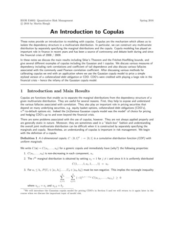
An Introduction to Copulas10Spearman’s rho is therefore simply the linear correlation of the probability-transformed random variables. TheSpearman’s rho matrix is simply the matrix of pairwise Spearman’s rho correlations, ρ(Fi (Xi ), Fj (Xj )). It is(why?) a positive-definite matrix. If X1 and X2 have continuous marginals then it can be shown thatZ 1 Z 1(C(u1 , u2 ) u1 u2 ) du1 du2 .ρs (X1 , X2 ) 1200It is also possible to show that for a bivariate Gaussian copula6ρarcsin' ρπ2where ρ is the Pearson, i.e., linear, correlation coefficient.ρs (X1 , X2 ) Definition 4 For random variables X1 and X2 , Kendall’s tau is defined ash iρτ (X1 , X2 ) : E sign (X1 X̃1 ) (X2 X̃2 )where (X̃1 , X̃2 ) is independent of (X1 , X2 ) but has the same joint distribution as (X1 , X2 ).Note that Kendall’s tau can be written as ρτ (X1 , X2 ) P (X1 X̃1 ) (X2 X̃2 ) 0 P (X1 X̃1 ) (X2 X̃2 ) 0so if both probabilities are equal then ρτ (X1 , X2 ) 0. If X1 and X2 have continuous marginals then it can beshown thatZ Z11C(u1 , u2 ) dC(u1 , u2 ) 1.ρτ (X1 , X2 ) 400It may also be shown that for a bivariate Gaussian copula, or more generally, if X E2 (µ, P, ψ) andP (X µ) 0 then2arcsin ρ(13)ρτ (X1 , X2 ) πwhere ρ P12 P21 is the Pearson correlation coefficient. We note that (13) can be very useful for estimatingρ with fat-tailed elliptical distributions. It generally provides much more robust estimates of ρ than the usualPearson estimator. This can be seen from Figure 2 where we compare estimates of Pearson’s correlation usingthe usual Pearson estimator versus using Kendall’s τ and (13). The true underlying distribution was bivariate twith ν 3 degrees-of-freedom and true Pearson correlation ρ 0.5. Each point in Figure 2 was an estimateconstructed from a sample of n 60 (simulated) data-points from the true distribution. We see the estimatorbased on Kendall’s tau is clearly superior to the usual estimator.Exercise 3 Can you explain why Kendall’s tau performs so well here? Hint: It may be easier to figure out whythe usual Pearson estimator can sometimes perform so poorly.Properties of Spearman’s Rho and Kendall’s TauSpearman’s rho and Kendall’s tau are examples of rank correlations in that, when the marginals are continuous,they depend only on the bivariate copula and not on the marginals. They are therefore invariant in this caseunder strictly increasing transformations.Spearman’s rho and Kendall’s tau both take values in [ 1, 1]: They equal 0 for independent random variables. (It’s possible, however, for dependent variables to alsohave a rank correlation of 0.) They take the value 1 when X1 and X2 are comonotonic. They take the value 1 when X1 and X2 are countermonotonic.As discussed in Section 4.3, Spearman’s rho and Kendall’s tau can be very useful for calibrating copulas viamethod-of-moments type algorithms. And as we have seen, the second fallacy associated with the Pearsoncoefficient is clearly no longer an issue when we work with rank correlations.

An Introduction to Copulas11Pearson Correlation10.50 0.5 105001000150020000500100015002000Kendall’s Tau10.50 0.5 1Figure 2: Estimating Pearson’s correlation using the usual Pearson estimator versus using Kendall’s τ .Underlying distribution was bivariate t with ν 3 degrees-of-freedom and true Pearson correlation ρ 0.5.3.2Tail DependenceWe have the following definitions of lower and upper tail dependence.Definition 5 Let X1 and X2 denote two random variables with CDF’s F1 and F2 , respectively. Then thecoefficient of upper tail dependence, λu , is given byλu : lim P (X2 F2 (q) X1 F1 (q))q%1provided that the limit exists. Similarly, the coefficient of lower tail dependence, λl , is given byλl : lim P (X2 F2 (q) X1 F1 (q))q&0provided again that the limit exists.If λu 0, then we say that X1 and X2 have upper tail dependence while if λu 0 we say they areasymptotically independent in the upper tail. Lower tail dependence and asymptotically independent in the lowertail are similarly defined using λl . The upper and lower coefficients are identical for both the Gaussian and tcopulas. Unless ρ 1 it can be shown that the Gaussian copula is asymptotically independent in both tails.This is not true of the t copula, however. In Figure 8.6 of Ruppert and Matteson (SDAFE, 2015) we haveplotted λl λu as a function of ρ for various values of the d.o.f, ν. It is clear (and makes intuitive sense) thatλl λu is decreasing in ν for any fixed value of ρ.

121.0An Introduction to Copulas0.60.40.00.2λl λu0.8ν 1ν 4ν 25ν 250 1.0 0.50.00.51.0ρFigure 8.6 from Ruppert and Matteson: Coefficients of tail dependence for bivariate t-copulas asfunctions of ρ for ν 1, 4, 25 and 250.4Estimating CopulasThere are several related methods that can be used for estimating copulas:1. Maximum likelihood estimation (MLE). It is often considered too difficult to apply as there too manyparameters to estimate.2. Pseudo-MLE of which there are two types: parametric pseudo-MLE and semi-parametric pseudo-MLE.Pseudo-MLE seems to be used most often in practice. The marginals are estimated via their empiricalCDFs and the copula is then estimated via MLE.3. Moment-matching methods are also sometimes used. They methods can also be used for findingstarting points for (pseudo)-MLE.We now discuss these methods in further detail.4.1Maximum Likelihood EstimationLet Y (Y1 . . . Yd ) be a random vector and suppose we have parametric models FY1 (· θ 1 ), . . . , FYd (· θ d )for the marginal CDFs. We assume that we also have a parametric model cY (· θ C ) for the copula density of Y.By differentiating (2) we see that the density of Y is given byfY (y) fY (y1 , . . . , yd ) cY (FY1 (y1 ), . . . , FYd (yd ))dYj 1fYj (yj ).(14)

An Introduction to Copulas13Suppose now that we are given an IID sample Y1:n (Y1 , . . . , Yn ). We then obtain the log-likelihood aslog L(θ 1 , . . . , θ d , θ C ) lognYfY (yi )i 1 n Xlog[cY (FY1 (yi,1 θ 1 ), . . . , FYd (yi,d θ d ) θ C )]i 1 log (fY1 (yi,1 θ 1 )) · · · log (fYd (yi,d θ d )) .(15)b1 , . . . , θbd , θbC are obtained by maximizing (15) with respect to θ 1 , . . . , θ d , θ C . There areThe ML estimators θproblems with this approach, however:1. There are (tto) many parameters to estimate, especially for large values of d. As a result, performing theoptimization can be difficult.2. If any of the parametric univariate distributions FYi (· θ i ) are misspecified then this can cause biases inthe estimation of both the univariate distributions and the copula.4.2Pseudo-Maximum Likelihood EstimationThe pseudo-MLE approach helps to resolve the problems associated with the MLE approach mentioned above.It has two steps:1. First estimate the marginal CDFs to obtain FbYj for j 1, . . . , d. We can do this using either: The empirical CDF of y1,j , . . . , yn,j so thatPnFbYj (y) 1{yi,j y}.n 1i 1bj obtained using the usual univariate MLE approach. A parametric model with θ2. Then estimate the copula parameters θ C by maximizingnXh ilog cY FbY1 (yi,1 ), . . . , FbYd (yi,d ) θ C(16)i 1Note that (16) is obtained directly from (15) by only including terms that depend on the (as yet) unestimatedparameter vector θ C and setting the marginals at their fitted values obtained from Step 1. It is worthmentioning that even (16) may be difficult to maximize if d large. In that event it is important to have a goodstarting point for the optimization or to impose additional structure on θ C .4.3Fitting Gaussian and t CopulasA moment-matching approach for fitting either the Gaussian or t copulas can be obtained immediately from thefollowing result.Proposition 7 (Results 8.1 from Ruppert and Matteson)Let Y (Y1 . . . Yd ) have a meta-Gaussian distribution with continuous univariate marginal distributions andGausscopula CΩand let Ωi,j [Ω]i,j . Thenρτ (Yi , Yj ) 2arcsin (Ωi,j )π(17) 6arcsin (Ωi,j /2) Ωi,jπ(18)andρS (Yi , Yj )tIf instead Y

the overall joint multivariate distribution can be di cult when it is constructed by separately specifying the marginals and copula. Nevertheless, an understanding of copulas is important in risk management. We begin with the de nition of a copula. De nition 1 A d-dimensional copula, C: [0;1