Transcription
Predictive Modelling Applied to Propensity toBuy Personal Accidents Insurance ProductsEsdras Christo Moura dos SantosInternship report presented as partial requirement forobtaining the Master’s degree in Advanced Analyticsi
2017Title: Predictive Models Applied to Propensity to Buy Personal AccidentsInsurance ProductsStudent: Esdras Christo Moura dos SantosMAAi
i
NOVA Information Management SchoolInstituto Superior de Estatística e Gestão de InformaçãoUniversidade Nova de LisboaPREDICTIVE MODELLING APPLIED TO PROPENSITY TO BUYPERSONAL ACCIDENTS INSURANCE PRODUCTSbyEsdras Christo Moura dos SantosInternship report presented as partial requirement for obtaining the Master’s degree inAdvanced AnalyticsAdvisor: Mauro Castelliii
February 2018DEDICATIONDedicated to my beloved family.iii
ACKNOWLEDGEMENTSI would like to express my gratitude to my supervisor, Professor Mauro Castelli of InformationManagement School of Universidade Nova de Lisboa for all the mentoring and assistance. I alsowant to show my gratitude for the data mining team at Ocidental, Magdalena Neate and FranklinMinang. I deeply appreciate all the guidance, patience and support during this project.iv
ABSTRACTPredictive models have been largely used in organizational scenarios with the increasingpopularity of machine learning. They play a fundamental role in the support of customer acquisitionin marketing campaigns. This report describes the development of a propensity to buy model forpersonal accident insurance products. The entire process from business understanding to thedeployment of the final model is analyzed with the objective of linking the theory to practice.KEYWORDSPredictive models; data mining; supervised learning; propensity to buy; logistic regression; decisiontrees; artificial neural networks; ensemble models.v
INDEX1. Introduction AND Motivation . 12. Part I. 22.1. Data Mining Processes . 22.1.1. CRISP-DM . 22.1.2. SEMMA . 42.2. Predictive Models . 62.2.1. Logistic Regression . 72.2.2. Decision Trees . 92.2.3. Artificial Neural Networks . 132.2.4. Ensemble Models . 162.3. Predictive Models Evaluation . 172.3.1. Performance Measure of Binary Classification . 173. Part II. 243.1. Methodology . 243.1.1. Business Understanding . 243.1.2. Data Understanding . 253.1.3. Data Preparation . 263.1.4. Modelling. 313.1.5. Final Evaluation and Results . 454. Conclusions and Deployment . 504.1. Limitations and Recommendations for Future Works . 50Appendix. 52Bibliography. 77vi
LIST OF FIGURESFigure 1 - CRISP-DM . 3Figure 2 - SEMMA . 4Figure 3 – Sigmoid Function. . 8Figure 4 – Decision Tree Representation. . 9Figure 5 – Logworth function. . 11Figure 6 – Entropy of a Binary Variable. 12Figure 7 - Artificial Neural Network Representation . 13Figure 8 – Sigmoid Activation Function. 15Figure 9 – ROC Curve . 22Figure 10 - Lift Chart . 23Figure 11 – Distribution of Idade Adj . 27Figure 12 – Distribution of No Claims Ever NH . 28Figure 13 – Sample Distribution of Idade-Adj . 29Figure 14 – Correlation Matrix . 30Figure 15 – Modelling Process. . 32Figure 16 - Regression Models . 33Figure 17 – Regression model Average Squared Error . 34Figure 18 – Regression ROC Curve . 35Figure 19 – Regression Misclassification Rate . 36Figure 20 – Decision Tree Models . 36Figure 21 – Decision Tree Average Squared Error . 38Figure 22 – Decision Tree Misclassification Rate . 39Figure 23 – Decision Tree ROC curves. . 39vii
Figure 24 – Decision Tree Structure . 40Figure 25 – Artificial Neural Networks Models . 41Figure 26 – Artificial Neural Network ASE with all inputs. . 41Figure 27 – Artificial Neural Network Average Squared Error. . 42Figure 28 – Artificial Neural Network Misclassification Rate. . 42Figure 29 – Artificial Neural Network ROC curves. . 43Figure 30 – Posterior Probabilities . 44Figure 31 – Ensemble Model ROC Curves . 45Figure 32 – Cummulative Lift Comparison . 46Figure 33 – Histogram of Unadjusted Probabilities. . 48Figure 34 – Histogram of Adjusted Probabilities. . 48Figure 35 – Decision Tree Structure. . 76viii
LIST OF TABLESTable 1 – CRISP-DM & SEMMA . 5Table 2 – Confusion Matrix . 17Table 3 – Data Partition. 29Table 4 – Regression Model Coefficients. . 34Table 5 – Regression Model Evaluation . 35Table 6 – Decision Tree Configuration . 38Table 7 – Decision Tree Evaluation . 38Table 8 – Artificial Neural Network Evaluation . 42Table 9 – Ensembel Model evaluation . 44Table 10 – Training Performance Comparison. . 46Table 11 – Validation Performance Comparison. . 46Table 12 – Probabilities statistics. . 47Table 13 – Test Data Cumulative Lift. . 49Table 14 –List of Input Variables . 59Table 15 – Variables excluded . 61Table 16 – Data set quantitative var. descriptive statistics. . 67Table 17 –Sample quantitative variables descriptive statistics . 73Table 18 – Statistics Comparison . 75ix
1. INTRODUCTION AND MOTIVATIONThe Master’s degree in Advanced Analytics at NOVA IMS offers the option of writing a thesis ordeveloping a practical project through an internship with the purpose of applying the theory studiedduring the first year of the master to earn the degree in Advanced Analytics. The aim of this report isto describe the development of a predictive model for understanding the propensity to buy aPersonal Accident Insurance product at Ocidental Seguros.One of the main reasons for studying predictive models is due to the enormous amount of datathat business produce today. As a result, the need to process this information to gain insights andmake improvements has become fundamental to stay competitive. The insurance industry is anexample of an industry that has taken advantage of analytics. One of the main objectives of aninsurance company, besides increasing its client base, is to increase the number of policies held by itsclients. Data mining techniques are applied to achieve this goal, especially predictive modelling.Predictive modelling is used in the marketing of many products and services. Insurers can usepredictive models to analyze the purchasing patterns of insurance customers in addition to theirdemographic attributes. This information can then be used to increase the marketing success rate,which is a measure of how often the marketing function generates a sale for each contact made witha potential customer. Predictive analytics used to analyze the purchasing patterns may allow theagents to focus on the customers who are more likely to buy, thereby increasing the success ofmarketing campaigns.This report is structured in two main parts. Part I is focused on the literature review andexplanation of the predictive modelling process, while Part II comprises the application of the theoryoutlined in the first section relating it to a practical business scenario. Additional businessspecifications are described to achieve this goal throughout the development of a predictive modelapplied to a propensity to buy personal accident insurance products.1
2. PART IDeveloping a predictive model it is one of the steps that are encompassed in the data miningprocess. As such, Part I of this report starts with a brief explanation of the data mining process andproceeds with the explanation of the predictive modelling task.2.1. DATA MINING PROCESSESBefore analyzing the techniques applied to predictive modelling, it is crucial to have an overviewof the whole data mining process. Two main methodologies with similar approaches are presentedbelow. Their applications are detailed in the practical section.2.1.1. CRISP-DMCRISP-DM1 (Olson & Delen, 2008) is a process widely used by the industry members. Thisprocess consists of six phases that can be partially cyclical (Figure 1):1Cross-Industry Standard Process for data mining2
Figure 1 - CRISP-DM Business Understanding: Most of the data mining processes aim to provide a solution to aproblem. Having a clear understanding of the business objectives, assessment of the currentsituation, data mining goals and the plan of development are fundamental to the achievementof the objectives. Data Understanding: Once the business context and objectives are covered, dataunderstanding considers data requirements. This step encompasses data collection and dataquality verification. At the end of this phase, a preliminary data exploration can occur. Data Preparation: In this step, the data cleaning techniques are applied to prepare the data tobe used as input for the modelling phase. A more thorough data exploration is carried duringthis phase providing an opportunity to see patterns based on business understanding. Modelling: The modelling stage uses data mining tools to apply algorithms suitable to the taskat hand. The next section of this report is dedicated to detail a few techniques applied duringthis step.3
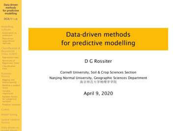
Evaluation: The evaluation of the models is done by taking into account several evaluationmetrics and comparing the performance of the models built during the modelling phase. Thisstep should also consider the business objectives when choosing the final model. Deployment: The knowledge discovered during the previous phases need to be reported tothe management and be applied to the business environment. Additionally, the insights gainedduring the process might change over time. Therefore, it is critical that the domain of interestbe monitored during its period of deployment.2.1.2. SEMMAIn addition to CRISP-DM, another well-known methodology developed by the SAS Institute is theSEMMA2 process (Olson & Delen, 2008) shown in Figure 2. Each phase of the process is describedbelow:Figure 2 - SEMMA Sample: Representative samples of the data are extracted to improve computationalperformance and reduce processing time. It is also appropriately partition the data intotraining validation and test data for better modelling and accuracy assessment; Explore: Through the exploration of the data, data quality is assured and insights are gainedbased on visualization and summary statistics. Trends and relationship can also be identified inthis step; Modify: Based on the discoveries during the exploration phase it might be necessary toexclude, create and transform the variables in the data set before the modelling phase. It is2Sample, Explore, Modify, Model and Assess4
also important to verify the presence of outliers, which can damage the performance of themodels; Model: During this phase, the search task of finding the model that best accomplish the goalsof the process is performed. The models might serve different purposes, but are generallyclassified into two groups. The first concerns the descriptive models, also known asunsupervised learning models, this set of techniques aim to describe the structure and/orsummarize the data. Clustering and association rules are examples of descriptive/unsupervisedalgorithms. The second group comprehends the predictive models, also known as supervisedlearning models, the objective of these models is to create structures that can predict withsome degree of confidence the outcome of an event based on a set of labeled examples. Amore precise definition is given in the next section; Assess: In this final step of the data mining process the user assesses the model to estimatehow well it performs. A common approach to assess the performance of the model is to applythe model to a portion of the data that was not used to build the model. Then, an unbiasedestimative of the performance of the model can be analyzed.The two data mining processes mentioned give an overview of the development of a predictivemodel. These two approaches were shown because the CRISP-DM relates the data mining processwith the business context, while SEMMA details the technical steps needed to build a model once thebusiness objectives have been defined. The table below (Table 1) shows the similarity between eachphase of both processes.CRISP-DMSEMMABusinessUnderstanding-Data UnderstandingSampleExploreData tDeployment-Table 1 – CRISP-DM & SEMMAAfter giving an overview of the data mining process, we can now concentrate on the modellingpart of the process. The next section is dedicated to describing the predictive models used during thepractical section.5
2.2. PREDICTIVE MODELSAs mentioned in the previous section, the modelling step of a project can have two approachesaccording to the objective, a predictive or descriptive modelling analysis. In this section, thepredictive models discussed are focused on a binary classification problem since it is the scenario ofthe practical section of this report. A few concise definitions of predictive modelling are presentedbelow.“Predictive modeling is a name given to a collection of mathematical techniques having incommon the goal of finding a mathematical relationship between a target, response, or “dependent”variable and various predictor or “independent” variables with the goal in mind of measuring futurevalues of those predictors and inserting them into the mathematical relationship to predict futurevalues of the target variable”(Dickey, D. A., 2012, Introduction to Predictive Modeling with Examples)“Predictive Analytics is a broad term describing a variety of statistical and analytical techniquesused to develop models that predict future events or behaviors. The form of these predictive modelsvaries, depending on the behavior or event they are predicting. Most predictive models generate ascore (a credit score, for example), with a higher score indicating a higher likelihood of the givenbehavior or event occurring”(Nyce C., 2007, Predictive Analytics White Paper)“Predictive modelling (also known as supervised prediction or supervised learning) starts with atraining data set. The observations in a training data set are known as training cases (also calledtraining examples, instances, or records). The variables are called inputs (also known as predictors,features, explanatory variables, or independent variables) and targets (also known as response,outcome, or dependent variable). For a given case, the inputs reflect your state of knowledge beforemeasuring the target”(Christie et al., 2011, Applied Analytics Using SAS Enterprise Miner)The definitions above state that predictive model is a relationship between a target variable anda set of inputs. This relationship is detected by analyzing the training data set. Additionally, otherdata sets are used to improve the performance of a predictive model and its ability to generalize forcases that are not in the training data, validation data and test data address this problem. Theformer is used to evaluate the error of the model and gives an indication when to stop training toimprove its generalization, while the latter is used exclusively to give an unbiased estimation of theperformance of the model.Regardless of the predictive model, it must fulfill the following requirements: Provide a rule to transform a measurement into a prediction; Be able to attribute importance among useful input from a vast number of candidates; Have a mean to adjust its complexity to compensate for noisy training data.6
In the following subsections, the three most commonly used predictive modelling methods anda combination of them are detailed, considering the implementations provided by the SAS EM3 datamining tool.2.2.1. Logistic RegressionLogistic Regression is a type of regression applied when the target variable is a dichotomous(binary) variable and it belongs to a class of models named GLM (generalized linear models). The goalof logistic regression is to estimate the probability of an event conditional to a set of input variables(Hosmer, Lemeshow, 1989). After estimating the probability of an instance, the classification of it asevent or non-event can be made.As mentioned previously, the target variable can take value 1 with probability of success p orvalue 0 with probability (1-p). Variables with this nature follow a Bernoulli distribution, which is aspecial case of the Binomial distribution when the number of trials is equal to 1. The relationshipbetween the target variable and the inputs is not a linear function in a logistic regression, a linkfunction denominated logit is used to establish the association between the inputs and the targetvariable.𝑙𝑜𝑔𝑖𝑡(𝑝) ln (𝑝)1 𝑝However, the probability p is unknown, it has to be estimated conditional to the inputs. As aresult, the following equation describes the relation between the probability and the inputs:𝑝ln () 𝛽̅ 𝑇 𝑋̅1 𝑝With some algebra, the relationship can be simplified as the equation below.𝑝̂ 11 𝑒 𝛽̅𝑇𝑋̅The term on the right side of the equality is known as logistic function. If we define u 𝛽̅ 𝑇 𝑋̅, therelationship between the sigmoid function f and u can be visualized in Figure 3. Large values of u givehigh values of the dependent variable (𝑝̂ f(u)), while high negative values of u give values of thedependent variable close to 0.The values of f(u) are interpreted as the estimated posteriorprobabilities3SAS Enterprise Miner7
Figure 3 – Sigmoid Function.The goal of logistic regression is to correctly predict the category of the outcome for individualcases using the most parsimonious model. The coefficients 𝛽̅ are estimated through maximumlikelihood, but the choice of the most parsimonious model is subject to a variable selection method.Essentially, the choice of an adequate model is based on the significance of the coefficientsassociated with the input variable. The first possibility of variable selection method is the BackwardsSelection, with this option the training begins with all candidate inputs and removes the inputs untilonly inputs with p-values determined by an F-test or t-test are lower than a predefined significancelevel, typically 0.05. The Forward Selection method starts with no input variable, the inputs areincluded in the model sequentially based on the significance of each variable. At each iteration, thevariable with the lowest p-value lower than the significance level is included in the model. Thisprocess is repeated until there are no more variables that fulfill this entry criterion. Lastly, theStepwise Selection starts as Forward Selection, but the removal of inputs is possible if an inputsbecomes non-significant through the iterations. This process continues until no variable meets theentry criterion or other stop condition is reached.The final model, depending on the selection method, can also be evaluated on the validationdata. An alternative for not relying exclusively on the statistical significance of the model consists ofevaluating the model at each step of the model selection. Then, the model with the highestperformance on the validation set is chosen regardless if any of the inputs is significant or not.8
2.2.2. Decision TreesDecision Trees are among the most popular predictive algorithms due to their structure andinterpretability. Additionally, they are applied in various fields, ranging from medical diagnosis tocredit risk.2.2.2.1. Decision Trees RepresentationDecision trees classify instances by sorting them down from the root node to a leaf node. Eachnode in the tree test an if-else rule of some variable of an observation, and each branch descendingfrom that node corresponds to one of the possible values of this attribute. This process is repeateduntil a leaf node is reached. Figure 4 represents this procedure.Figure 4 – Decision Tree Representation.The first rule, at the base (top) of the tree, is named the root node. Subsequent rules are namedinterior nodes. Nodes with only one connection are leaf nodes. A tree leaf provides a classificationand an estimate (for example, the proportion of success events). A node, which is divided into subnodes is called parent node of sub-nodes, whereas sub-nodes are the child of parent node (Rokach &Maimon, 2015).2.2.2.2. Growing a Decision TreeThe growth of a decision tree is determined by a split-search algorithm. To measure thegoodness of a split different functions can be used, the most known are Entropy and Chi-Square, bothapproaches are available in SAS EM.9
2.2.2.3. CHAID (Chi-Square Automatic Interaction Detection)The splitting criterion in CHAID is based on the p-value of the Pearson Chi-Square ofIndependence, which defines the null hypothesis as the absence of a relation between theindependent variable and the target variable. By selecting the input variable with the lowestsignificant p-value, the algorithm is intrinsically selecting the variable that has the highest associationwith the target variable at each step (Ritschard, 2010).This algorithm has two steps:1) Merge step: The aim of this step is to group the categories that are not significantly differentfor each input variable. For example, if a nominal variables X1 has levels c1, c2 and c3. Then, achi-square test for each pair of levels is computed. The test with the highest p-value indicateswhat levels should be aggregated. This process repeats until only significantly aggregatedlevels are eligible for splitting;2) Split search: In this step, each input resulting from the previous step is considered for split.Then, for each input, the algorithm searches for the best split. That is, the point (or the classesfor nominal variables) that maximizes the logworth function. The logworth of a split is afunction of the p-value associated with the Chi-Square test of the input obtained in theprevious step and the target variable, it is given by the following equation:𝑙𝑜𝑔𝑤𝑜𝑟𝑡ℎ log10 (𝐶ℎ𝑖 𝑆𝑞𝑢𝑎𝑟𝑒𝑑 𝑝 𝑣𝑎𝑙𝑢𝑒)The input that provides the highest logworth is selected for split. Then, another split iscalculated if no termination criterion is met.The termination criteria in CHAID trees are the following:1) No split produce a logworth higher than the threshold defined;2) Maximum tree depth is reached;3) Minimum number of cases in a node for being a parent node is reached, so it cannot split anyfurther;4) Minimum number of cases in a node for being a child node is reached.10
In SAS EM the default value for comparison of the logworth is 0.7, which is associated with a pvalue of 0.2. Then, if an input has a logworth higher than 0.7, it is eligible to be used in a split. Thelogworth function can be analyzed in Figure 5, the dashed line represents the threshold.Figure 5 – Logworth function.2.2.2.4. Impurity Based TreesDifferently from the Chi-Square splitting criterion, which is based on statistical hypothesistesting, the entropy reduction criterion is related to information theory. Entropy measures theimpurity of a sample. The entropy function E of a collection S in a c class classification is defined as:E(S) 𝑐𝑖 1 𝑝𝑖 𝑙𝑜𝑔2 (𝑝𝑖 )Where 𝑝𝑖 is the proportion of S belonging to class 𝑖. For a binary target variable S, the entropyfunction is displayed in Figure 6 and it is computed as:E(S) [𝑝 𝑙𝑜𝑔2 (𝑝) (1 𝑝) 𝑙𝑜𝑔2 (1 𝑝)]11
Figure 6 – Entropy of a Binary VariableFigure 6 shows the variation of the entropy for a binary target variable. The maximum is reachedwhen there is no distinction for the target variable, which corresponds to a 50%-50% proportion ofevent and non-event. As a result, the aim of the algorithm is to find the split that minimizes theentropy, which provides the largest difference in proportion between the target levels.Entropy measures the impurity of a split in the training examples. To define the effectiveness ofa variable in classifying the training data the algorithm uses a measure called information gain (Gain),which is the reduction in entropy caused by the p
proceeds with the explanation of the predictive modelling task. 2.1. DATA MINING PROCESSES Before analyzing the techniques applied to predictive modelling, it is crucial to have an overview of the whole data mining process. Two main methodologies with similar approaches are presented below. Their applications are detailed in the practical .