WIXLIB

xviDistributional properties — the Weibull distribution122Distributional properties — type 1 extreme value distribution123Distributional properties — Cauchy distribution124Distributional properties — sine distribution125Distributional properties — normal distribution126Distributional properties — the standard logistic distribution156Distributional properties — the skew logistic distribution156Shapes of the standard symmetric lambda distribution159Distribution properties — symmetric lambda distribution159Distributional properties — four-parameter lambda distribution 160Shapes and properties of the canonical generalized lambda161Classes of generalized lambda distributions162Commonly available quantile functions170General shape plots175Plots for indicating skewness176Tail-shape plots176Tail values for some common distributions178Identification plots for positive distributions180Identification plots for distributions on (– , )181Layout for sample-population comparisons — example182Model selection by correlation184Illustrative layout for forward selection187Matching methods of estimation194Layout of DLS calculation for Q(p) λ ηS(p;β)201Fitting by the method of least absolutes202Fitting by the method of weighted least absolutes205Algorithm for least/maximum methods210Layout for fitting by maximum likelihood211 2000 by Chapman & Hall/CRC

xviiObtaining 100p% likelihood intervals216Example of % criterion ratio for sum of absolutes criterion216Significant values of the likelihood ratio, Rmin234Validating algorithm for least/maximum methods(y validation data)234Least squares fitting — crow–car data253Least absolutes fitting of a regression quantilefunction — crow–car data (normal model)257Fitting a linear regression quantile model259Least absolutes fitting of regression quantilefunction — crow–car data (Weibull model)264Algorithm for fitting a circular model282Algorithm for fitting a marginal-conditional model— bivariate logistic283Layout for fitting a bivariate logistic284Additional algorithm for a combined methodfor marginal/conditional models284 2000 by Chapman & Hall/CRC

PrefaceIn the early 1980s while working on a book on statistical modelling(Gilchrist (1984)), I came across a distribution called the generalizedlambda distribution. I duly mentioned it in passing, (p. 45), observing that it was defined in a different manner than the other distributions dealt with in the book. Later on, while working with students on placement with Glaxo-Chem and in other work with GlaxoWellcome, the opportunity arose to become familiar with the practical use of this highly flexible distribution. It slowly dawned onme, from this work and beginning to read the scattered literatureof relevance, that the evident practical value of the methods usedwas not just a matter of one distribution but of a particular way oflooking at statistical modelling. As a result, the ideas in this bookwere slowly put together. The book is not intended as a researchmonograph, but rather as a straightforward introductory text forpractitioners of statistical modelling. However, the approachadopted is different than the standard approach, as was taken inthe previous book, and leads to different definitions of even basicquantities like the mean. Thus, in many ways we are forced to goback to basics and look at statistical modelling from the beginning.We look, however, from a different perspective, which is notintended as a replacement to the classical approaches to modellingbut as a useful supplement, and indeed it will be seen that thereare many overlaps.I would like to thank the following individuals: staff from Sheffield Hallam University, especially Dr Steve Salter, Richard Gibson,and Penny Veitch; Professor Emanuel Parzen for his helpful comments and particularly for the idea of starting with an overviewchapter; staff from the Glaxo Wellcome Group, particularly Dr MaxPorter and Miss Gillian Amphlett; Dr Alan Hutson and James Meginniss for their many helpful comments on the penultimate draft text(although any errors in the final text are my responsibility); and my 2000 by Chapman & Hall/CRC

xxwife for her support and her patience with a husband who is supposedto be retired.Warren GilchristJanuary 2000w.g.gilchrist@shu.ac.uk 2000 by Chapman & Hall/CRC

CHAPTER 1An Overview1.1IntroductionIn the balance of this book we will look systematically at the manyissues associated with the steps of the statistical modelling process,using an approach based on what will be termed quantile methods.However, there is the danger that, if we do just go through thesemethods step by step, the reader will not see the wood for the trees.The aim of this chapter is thus to provide an outline of the wood. Thiswill be done by bringing together the simplest of the ideas andapproaches of quantile modelling to form both an initial picture anda basis for later development.Anyone who has studied statistics, even at the most basic level,will have already met quantile methods, although may not be awareof it. A quantile is simply the value that corresponds to a specifiedproportion of a sample or population. Thus the median of a sample ofdata is the quantile corresponding to a proportion 0.5 of the ordereddata. For a theoretical population it corresponds to the quantile withprobability of 0.5. If Q(p) is the function, called the quantile function,that gives the quantile values for all probabilities p, 0 p 1, thenthe median is Q(0.5). Similarly, we have the quartiles Q(1/4) andQ(3/4). Most users of statistics will have utilized tables of the normaldistribution to look up, for example, values such as 1.96 as the valuethat has a probability of 0.975 of not being exceeded. Thus if N(p) isthe quantile function for the standard normal distribution then 1.96is N(0.975), so the normal tables used are just the tables of the quantilefunction for the standard normal distribution.What is the link then to modelling? The fact that in the lastdiscussion a standard normal quantile function was used implied thatthere was some prior modelling to justify the use of the normal distributional model rather than any one of the multitudes of alternatives.The fact that a standard normal distribution was used required some 2000 by Chapman & Hall/CRC

2AN OVERVIEWmatching of the data being studied to the normal distribution model.Almost all practical statistics imply some form of modelling.We will study these ideas again more carefully later. But we stillhave not said why an entire book needs to be devoted to linking theideas of quantile functions to the process of statistical modelling. Thereare two prime reasons:1.2.Statistical modelling is a tool used essentially as part ofproblem solving. The purpose of having a statistical modelis almost always to assist in some problem-solving activity.The model assists in carrying out a prediction; it is used insome selection process or it helps in answering some “whatif ?” question. Modelling is part of the problem solvingprocess. A well-recognised feature of problem solving is thatproblems are often solved by seeking alternative ways oflooking at the problem. For example, where data is a seriesof observations in time, the classical models use a timeorigin, t 0, that is a fixed point in time. If, however, t 0is a moving time, e.g., it is always t now, then a new rangeof models become available for studying the problems oftime series. It will be seen repeatedly through the pages ofthis book that expressing statistical ideas in terms of quantile functions gives both a new perspective and sometimesa simpler and clearer perspective. Thus an approach basedon quantile functions provides an additional perspective forthe problem solver in the use of statistical models.Many statistical models consist of deterministic and stochastic (chance, random) elements. The classical approachto statistical modelling is such that the deterministic element is often built up by adding together, or sometimesmultiplying, simple components, as with a construction kitlike Lego . The stochastic element, however, is usuallychosen from a library of distributional models that has beenbuilt up over the last few centuries and is described in suchbooks as Johnson, Kotz and Balakrishnan (1994 and 1995)and Evans, Hastings and Peacock (1993). We will see thatif the stochastic element is modelled using quantile functions, then both elements in the model can be developedwith a common construction kit approach. In the same waythat deterministic modelling is a construction process so,too, using quantile functions is distributional modelling.Together there is a unified approach to model construction. 2000 by Chapman & Hall/CRC

THE DATA AND THE MODEL3For the rest of this text we will amplify and explore these two ideas.For now, however, let us start at the beginning.1.2The data and the modelStatistics has to start with data, a set of numbers collected in someexperiment, survey or observational study. Sometimes a simple studyof the data may seem to tell us what we want to know. We can drawplots of the data and work out average values and get a feel for thesituation being studied. However, one feature that is almost universally present in data is its variability. In addition to the factors inthe situation of which we are aware, there will be many other chanceinfluences jostling data values away from the perfect information wewould like to have. We are forced to recognise that if we repeatedthe exercise we would not get a repeat of the same set of data. Wethus have to speak of the data obtained as being a sample from apopulation of possible values. The language reflects the early useof a sample of people being measured as representative of the wholepopulation of a country. It is hoped, for example, that a large randomsample will clearly and accurately show the features of the populationof interest. We can describe the sample using graphs and summarynumbers, such as the average. To describe the population we needthe concept of the model, which is usually a mathematical description of the features of interest. Over the centuries, vast ranges ofmathematically based models have been developed to cover situationsin both sciences and social sciences. These models often consist oftwo components. First, there is a deterministic element whichdescribes behaviour or relationship with no allowance for chance orvariability. Second, there is the random element that allows for theinfluence of the uncertainty inherent in almost all situations. Thefocus of this book is on the forms that the random element may take,although in Chapter 12 we look at the construction of models thatinvolve the two elements.1.3Sample propertiesBefore we can sensibly model a set of data we need to have a clearperception of it, otherwise we will find ourselves imposing our views ofhow it ought to behave, rather than finding out how it does behave. The 2000 by Chapman & Hall/CRC

4AN OVERVIEWbest way to develop this perception and feel for the data is graphically,with the support of some numerical summaries of the properties seenon the graphs. Failure to link the graphs and summaries can result inthe use of summaries that are meaningless or misleading for the databeing analyzed. Let us look at a set of data to illustrate a number ofdifferent approaches.Example 1.1: Table 1.1 gives the layout for a calculation based on themaximum flow of flood water on a river for 20 periods of 4 years, inmillion cu. ft. per sec. The data are given and studied in Dumonceauxand Antle (1973). There are no strong features over time so the distributional features of the whole set of data will be used for illustration,although we will return to this issue later. The original data has beensorted by magnitude and placed in the column headed x. This is afundamental step in the types of analysis that will be developed in thistext. It is the ‘shape’ of the ordered data that describes its structure.With each ordered value, x, we will associate a probability p, indicatingthat the x lies a proportion, p, of the way through the data. At first guesswe would associate the rth ordered observation, denoted by x(r), with 0.050.050.050.050.050.050.05n 97Table 1.1. Layout for flood data plots 2000 by Chapman & 5.005.0012.525.0010.001.921.435.000.421.220.58

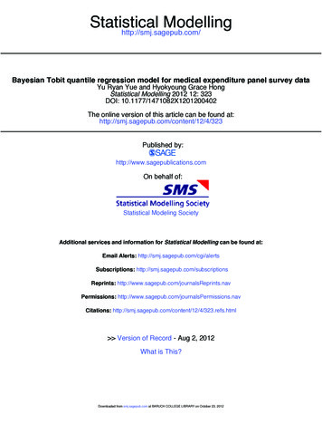
SAMPLE PROPERTIESFigure 1.1. (a) Flood data — x against p; (b) Flood data — p against x r/n, n 20, r 1, ,20. However, the range of values we would expectfor p is (0, 1). The value of r/n, however, goes from 1/20 to 1, i.e., it isnot symmetrical. Hence, to get the p values symmetrically placed in theinterval (0, 1), we use the formula pr (r – 0.5)/n. This formula corresponds to breaking the interval (0, 1) into 20 equal sections and usingthe midpoint of each. Thus we have pairs of values describing the dataas (x(r), pr). The value of x for any p is referred to as the sample pquantile. There are two natural plots of such data. First, of x(r) againstpr, and second, of pr against x(r), which are just the same plot with the 2000 by Chapman & Hall/CRC5

6AN OVERVIEWaxes interchanged. However, a look at these plots in Figure 1.1(a) and(b) shows that different features stand out most clearly in different plots.For x against p, there is a steady increase in x that becomes a steeperincrease towards the higher values of p. For the plot of p against x, thechange in the slope of p with x looks more dramatic, as does the breakin the data. The break is due to two of the ordered observations beingsomewhat further apart than those around them. This is almost certainlya chance feature and often occurs in such plots. The difference in slopebetween high values and low values of x looks to be a much more naturalfeature of the data.The discussion of slopes suggests that the slopes themselves be plotted.Thus if Dx is the difference between two successive values of the orderedx, called spacings, and Dp is the difference in their p values, then wecan derive a set of 19 pairs (Dx,Dp). The calculation is shown inTable 1.1 and the consequent slopes Dx/Dp and Dp/Dx calculated. Figure1.2(a) shows Dp/Dx plotted against the mid-values of the two xs usedfor each Dx. Figure 1.2(b) shows the values of Dx/Dp plotted againstthe mid-values of the two ps used for each Dp. In Figure 1.2(a), thepoints are linked to form a polygon. Linking successive points is aprocedure that sometimes helps, and sometimes hinders, seeing thedata. The high peak is due to two x values being particularly closetogether. The plot shows a great deal of random behaviour, but alsosome structure, with the higher values being around 0.4 and a straggling tail to the right. The plot of Dx/Dp against p shows low valuesover the central third of the probability and higher values at theextremes, particularly to the right. One final variant used in plottingthese quantities is to plot Dp/Dx, not against x, but against p. This plotshows how the rate of change in the probability is modified accordingto how far, proportionately, the observations are through the data, asFigure 1.3 illustrates.The problem of the randomness exhibited by Dp/Dx is partially dealtwith here by a process of smoothing the data. We deal with the detailof this later. It clearly helps the picturing of the situation, at the cost ofsome distortion. This group of five plots illustrates the points that (a)in any set of data, particularly when there are as few as 20 observations,there will be many results of sheer randomness in the data; (b) differentplots will show most clearly different features of the data; (c) in spite ofthe randomness, there are features, structures, in the data that the usercan seek to study and describe.Before leaving the data presented in Table 1.1, it should be noted thatduring the course of this book we will often show the layouts for calculations, sometimes just a section of a bigger table for illustration. The 2000 by Chapman & Hall/CRC

SAMPLE PROPERTIES7Figure 1.2. (a) Flood data — Dp/Dx against mid-x; (b) Flood data — Dx/Dp againstmid-papproach throughout is to present statistical calculations in columnform. This approach is regarded as essential for building a feel for boththe data and the models being used. It also facilitates the plotting ofgraphs, another central emphasis in our studies.In addition to graphical studies of data it is useful to have some summaryvalues that give a numerical indication of the shape of the data. Thesimplest of these is the sample median, m, which is the mid-value inthe data. With the even number of observations in Table 1.1 the median 2000 by Chapman & Hall/CRC

8AN OVERVIEWsmoothed Dp/Dx321000.20.4p0.60.81Figure 1.3. Flood data — smoothed Dp/Dx against mid-pis taken to be midway between the tenth and eleventh observations, som (0.402 0.412)/2 0.407. The values one quarter and three quartersof the way through the data are called the sample lower quartile andupper quartile, respectively, lq and uq. For Table 1.1 these will againlie between data points. We use the halfway point for now, but discussthe matter further later. Thus lq (0.3225 0.338)/2, which is 0.330.Similarly, uq 0.4665.Two measures of the shape of the data can be derived from the quartiles.The first is the interquartile range, iqr, which is simply the differencebetween the two quartiles, iqr uq – lq. For Table 1.1, this is 0.136.The iqr gives a simple measure of the spread of the data. Parzen (1997)suggests the quartile deviation, defined as 2iqr, as a more suitablequantity for some purposes. The range, w, of the data is the total spreadfrom smallest to largest observation, which in our case is 0.475. For asymmetrically shaped distribution, the deviations of the quartiles fromthe median will be approximately the same. Thus the difference betweenthese deviatio

1.4 Modelling the population 9 The cumulative distribution function 9 The probability density function 11 The quantile function 12 The quantile density function 14 1.5 A modelling kit for distributions 15 1.6 Modelling with quantile functions 17 1.7 Simple properties of population