Transcription
A Beginner’s Guide to High–Performance Computing1Module DescriptionDeveloper: Rubin H Landau, Oregon State University, http://science.oregonstate.edu/ rubin/Goals: To present some of the general ideas behind and basic principles of high–performance computing (HPC) as performed on a supercomputer. These concepts should remain valid even as thetechnical specifications of the latest machines continually change. Although this material is aimedat HPC supercomputers, if history be a guide, present HPC hardware and software become desktopmachines in less than a decade.Outcomes: Upon completion of this module and its tutorials, the student should be able to Understand in a general sense the architecture of high performance computers. Understand how the the architecture of high performance computers affects the speed ofprograms run on HPCs. Understand how memory access affects the speed of HPC programs. Understand Amdahl’s law for parallel and serial computing. Understand the importance of communication overhead in high performance computing. Understand some of the general types of parallel computers. Understand how different types of problems are best suited for different types of parallelcomputers. Understand some of the practical aspects of message passing on MIMD machines.Prerequisites: Experience with compiled language programming. Some familiarity with, or at least access to, Fortran or C compiling. Some familiarity with, or at least access to, Python or Java compiling. Familiarity with matrix computing and linear algebra.1
Intended Audience: Upper–level undergraduates or graduate students.Teaching Duration: One-two weeks. A real course in parallel computing would of course be atleast a full term.Activities: There is considerable material to be read concerning HPC concepts and terms thatare important to understand for a general understanding of HPC. Learning the semantics is animportant first step. The tutorial part of the module demonstrates and leads the reader throughsome techniques for writing programs that are optimized for HPC hardware. The reader experiments with their computer’s memory and experiences some of the concerns, techniques, rewards,and shortcomings of HPC.Student Assessment: The first element to student assessment would be to determine if theyunderstand the semantics. Understanding the importance of memory access on program speed, andparticularly the importance of paging and communication would be the next level of assessment.Actually being able to optimize programs for HPC hardware might be beyond the capability ofmost undergraduates, but important for research–oriented students.Testing: The materials have been developed and used for teaching in Computational Physics classesand at seminars for many years. They have also been presented at tutorials at SC conferences.Feedback from students involved with research has been positive.Contents1 Module Description12 High–Performance Computers33 Memory Hierarchy44 The Central Processing Unit75 CPU Design: Reduced Instruction Set Computers76 CPU Design: Multiple–Core Processors87 CPU Design: Vector Processors98 Introduction to Parallel Computing109 Parallel Semantics (Theory)1210 Distributed Memory Programming1411 Parallel Performance1511.1 Communication Overhead . . . . . . . . . . . . . . . . . . . . . . . . . . . . . . . . . 1712 Parallelization Strategies182
13 Practical Aspects of MIMD Message Passing1913.1 High–Level View of Message Passing . . . . . . . . . . . . . . . . . . . . . . . . . . . 2014 Scalability2214.1 Scalability Exercises . . . . . . . . . . . . . . . . . . . . . . . . . . . . . . . . . . . . 2315 Data Parallelism and Domain Decomposition2415.1 Domain Decomposition Exercises . . . . . . . . . . . . . . . . . . . . . . . . . . . . . 2716 The IBM Blue Gene Supercomputers2817 Towards Exascale Computing via Multinode–Multicore–GPU Computers2918 General HPC Program Optimization3118.1 Programming for Virtual Memory . . . . . . . . . . . . . . . . . . . . . . . . . . . . 3118.2 Optimizing Programs; Python versus Fortran/C . . . . . . . . . . . . . . . . . . . . 3218.2.1 Good, Bad Virtual Memory Use . . . . . . . . . . . . . . . . . . . . . . . . . 3319 Empirical Performance of Hardware3419.1 Python versus Fortran/C . . . . . . . . . . . . . . . . . . . . . . . . . . . . . . . . . 3520 Programming for the Data Cache (Method)4120.1 Exercise 1: Cache Misses . . . . . . . . . . . . . . . . . . . . . . . . . . . . . . . . . . 4220.2 Exercise 2: Cache Flow . . . . . . . . . . . . . . . . . . . . . . . . . . . . . . . . . . 4320.3 Exercise 3: Large-Matrix Multiplication . . . . . . . . . . . . . . . . . . . . . . . . . 4321 Practical Tips for Multicore, GPU Programming244High–Performance ComputersHigh performance and parallel computing is a broad subject, and our presentation is brief and givenfrom a practitioner’s point of view. Much of the material presented here is taken from A Survey ofComputational Physics, coauthored with Paez and Bordeianu [LPB 08]. More in depth discussionscan be found in the text by Quinn [Quinn 04], which surveys parallel computing and MPI from acomputer science point of view, and especially the references [Quinn 04, Pan 96, VdeV 94, Fox 94].More recent developments, such as programming for multicore computers, cell computers, andfield–programmable gate accelerators, are discussed in journals and magazines [CiSE], with a shortdiscussion at the end.By definition, supercomputers are the fastest and most powerful computers available, and atpresent the term refers to machines with hundreds of thousands of processors. They are the superstars of the high–performance class of computers. Personal computers (PCs) small enough in sizeand cost to be used by an individual, yet powerful enough for advanced scientific and engineeringapplications, can also be high–performance computers. We define high–performance computers asmachines with a good balance among the following major elements: Multistaged (pipelined) functional units. Multiple central processing units (CPUs) (parallel machines). Multiple cores.3
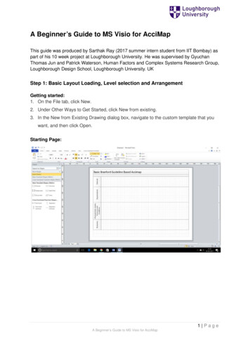
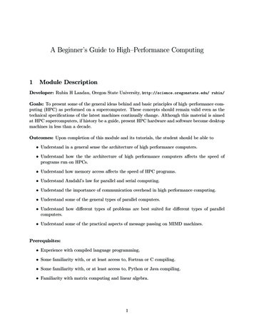
(2,2)M(3,2)M(N,N)Figure 1: The logical arrangement of the CPU and memory showing a Fortran array A(N ) andmatrix M (N, N ) loaded into memory. Fast central registers. Very large, fast memories. Very fast communication among functional units. Vector, video, or array processors. Software that integrates the above effectively.As a simple example, it makes little sense to have a CPU of incredibly high speed coupled to amemory system and software that cannot keep up with it.3Memory HierarchyAn idealized model of computer architecture is a CPU sequentially executing a stream of instructionsand reading from a continuous block of memory. To illustrate, in Figure 1 we see a vector A[ ] andan array M[ ][ ] loaded in memory and about to be processed. The real world is more complicatedthan this. First, matrices are not stored in blocks but rather in linear order. For instance, in Fortranit is in column–major order:M (1, 1) M (2, 1) M (3, 1) M (1, 2) M (2, 2) M (3, 2) M (1, 3) M (2, 3) M (3, 3),while in Python, Java and C it is in row–major order:M (0, 0) M (0, 1) M (0, 2) M (1, 0) M (1, 1) M (1, 2) M (2, 0) M (2, 1) M (2, 2).Second, as illustrated in Figures 2 and 3, the values for the matrix elements may not even be inthe same physical place. Some may be in RAM, some on the disk, some in cache, and some inthe CPU. To give some of these words more meaning, in Figures 2 and 3 we show simple modelsof the memory architecture of a high–performance computer. This hierarchical arrangement arisesfrom an effort to balance speed and cost with fast, expensive memory supplemented by slow, lessexpensive memory. The memory architecture may include the following elements:4
A(1)A(2)A(3)Data CacheA(1).A(16)A(2032) .RAMPage 1A(2048)A(N)M(1,1)M(2,1)M(3,1)Page 2M(N,1)M(1,2)M(2,2)M(3,2)Swap SpaceCPURegistersPage 3Page NM(N,N)GB32Main StoreBMTB32Paging Storage Controller2RAM2CPUcachekBFigure 2: The elements of a computer’s memory architecture in the process of handling matrixstorage.Figure 3: Typical memory hierarchy for a single–processor, high–performance computer (B bytes,K, M, G, T kilo, mega, giga, tera).CPU: Central processing unit, the fastest part of the computer. The CPU consists of a number ofvery–high–speed memory units called registers containing the instructions sent to the hardware to do things like fetch, store, and operate on data. There are usually separate registersfor instructions, addresses, and operands (current data). In many cases the CPU also containssome specialized parts for accelerating the processing of floating–point numbers.Cache: A small, very fast bit of memory that holds instructions, addresses, and data in theirpassage between the very fast CPU registers and the slower RAM. (Also called a high–speedbuffer.) This is seen in the next level down the pyramid in Figure 3. The main memory is alsocalled dynamic RAM (DRAM), while the cache is called static RAM (SRAM). If the cache isused properly, it can greatly reduce the time that the CPU waits for data to be fetched frommemory.Cache lines: The data transferred to and from the cache or CPU are grouped into cache or datalines. The time it takes to bring data from memory into the cache is called latency.5
RAM: Random–access or central memory is in the middle of the memory hierarchy in Figure 3.RAM is fast because its addresses can be accessed directly in random order, and because nomechanical devices are needed to read it.Pages: Central memory is organized into pages, which are blocks of memory of fixed length. Theoperating system labels and organizes its memory pages much like we do the pages of a book;they are numbered and kept track of with a table of contents. Typical page sizes are from 4to 16 kB, but on supercomputers may be in the MB range.Hard disk: Finally, at the bottom of the memory pyramid is permanent storage on magneticdisks or optical devices. Although disks are very slow compared to RAM, they can store vastamounts of data and sometimes compensate for their slower speeds by using a cache of theirown, the paging storage controller.Virtual memory: True to its name, this is a part of memory you will not find in our figuresbecause it is virtual. It acts like RAM but resides on the disk.When we speak of fast and slow memory we are using a time scale set by the clock in the CPU.To be specific, if your computer has a clock speed or cycle time of 1 ns, this means that it couldperform a billion operations per second if it could get its hands on the needed data quickly enough(typically, more than 10 cycles are needed to execute a single instruction). While it usually takes1 cycle to transfer data from the cache to the CPU, the other types of memories are much slower.Consequently, you can speed up your program by having all needed data available for the CPUwhen it tries to execute your instructions; otherwise the CPU may drop your computation and goon to other chores while your data gets transferred from lower memory (we talk more about thissoon in the discussion of pipelining or cache reuse). Compilers try to do this for you, but theirsuccess is affected by your programming style.As shown in Figure 2 for our example, virtual memory permits your program to use more pagesof memory than can physically fit into RAM at one time. A combination of operating system andhardware maps this virtual memory into pages with typical lengths of 4–16 kB. Pages not currentlyin use are stored in the slower memory on the hard disk and brought into fast memory only whenneeded. The separate memory location for this switching is known as swap space (Figure 2).Observe that when the application accesses the memory location for M[i][j], the number of thepage of memory holding this address is determined by the computer, and the location of M[i][j]within this page is also determined. A page fault occurs if the needed page resides on disk ratherthan in RAM. In this case the entire page must be read into memory while the least recently usedpage in RAM is swapped onto the disk. Thanks to virtual memory, it is possible to run programson small computers that otherwise would require larger machines (or extensive reprogramming).The price you pay for virtual memory is an order-of-magnitude slowdown of your program’s speedwhen virtual memory is actually invoked. But this may be cheap compared to the time you wouldhave to spend to rewrite your program so it fits into RAM or the money you would have to spendto buy a computer with enough RAM for your problem.Virtual memory also allows multitasking, the simultaneous loading into memory of more programs than can physically fit into RAM (Figure 4). Although the ensuing switching among applications uses computing cycles, by avoiding long waits while an application is loaded into memory,multitasking increases the total throughout and permits an improved computing environment forusers. For example, it is multitasking that permits a windowing system, such as Linux, OS X orWindows, to provide us with multiple windows. Even though each window application uses a fairamount of memory, only the single application currently receiving input must actually reside in6
BADCFigure 4: Multitasking of four programs in memory at one time in which the programs are executedin round–robin order.Table 1: Computation of c (a b)/(d f )Step 2Step 3Step 4Fetch bAdd—Arithmetic UnitA1Step 1Fetch aA2Fetch dFetch fMultiply—A3———Dividememory; the rest are paged out to disk. This explains why you may notice a slight delay whenswitching to an idle window; the pages for the now active program are being placed into RAM andthe least used application still in memory is simultaneously being paged out.4The Central Processing UnitHow does the CPU get to be so fast? Often, it employs prefetching and pipelining; that is, it has theability to prepare for the next instruction before the current one has finished. It is like an assemblyline or a bucket brigade in which the person filling the buckets at one end of the line does not waitfor each bucket to arrive at the other end before filling another bucket. In the same way a processorfetches, reads, and decodes an instruction while another instruction is executing. Consequently,even though it may take more than one cycle to perform some operations, it is possible for data tobe entering and leaving the CPU on each cycle. To illustrate, Table 1 indicates how the operationc (a b)/(d f ) is handled. Here the pipelined arithmetic units A1 and A2 are simultaneouslydoing their jobs of fetching and operating on operands, yet arithmetic unit A3 must wait for thefirst two units to complete their tasks before it has something to do (during which time the othertwo sit idle).5CPU Design: Reduced Instruction Set ComputersReduced instruction set computer (RISC) architecture (also called superscalar ) is a design philosophy for CPUs developed for high-performance computers and now used broadly. It increases thearithmetic speed of the CPU by decreasing the number of instructions the CPU must follow. Tounderstand RISC we contrast it with complex instruction set computer (CISC), architecture. Inthe late 1970s, processor designers began to take advantage of very-large-scale integration (VLSI),which allowed the placement of hundreds of thousands of devices on a single CPU chip. Much ofthe space on these early chips was dedicated to microcode programs written by chip designers andcontaining machine language instructions that set the operating characteristics of the computer.There were more than 1000 instructions available, and many were similar to higher–level programming languages like Pascal and Forth. The price paid for the large number of complex instructions7
was slow speed, with a typical instruction taking more than 10 clock cycles. Furthermore, a 1975study by Alexander and Wortman of the XLP compiler of the IBM System/360 showed that about30 low–level instructions accounted for 99% of the use with only 10 of these instructions accountingfor 80% of the use.The RISC philosophy is to have just a small number of instructions available at the chip levelbut to have the regular programmer’s high level–language, such as Fortran or C, translate theminto efficient machine instructions for a particular computer’s architecture. This simpler scheme ischeaper to design and produce, lets the processor run faster, and uses the space saved on the chip bycutting down on microcode to increase arithmetic power. Specifically, RISC increases the numberof internal CPU registers, thus making it possible to obtain longer pipelines (cache) for the dataflow, a significantly lower probability of memory conflict, and some instruction–level parallelism.The theory behind this philosophy for RISC design is the simple equation describing the execution time of a program:CPU time number of instructions cycles/instruction cycle time.(1)Here “CPU time” is the time required by a program, “number of instructions” is the total number ofmachine–level instructions the program requires (sometimes called the path length), “cycles/instruction” is the number of CPU clock cycles each instruction requires, and “cycle time” is the actualtime it takes for one CPU cycle. After viewing (1) we can understand the CISC philosophy, whichtries to reduce CPU time by reducing the number of instructions, as well as the RISC philosophy,which tries to reduce the CPU time by reducing cycles/instruction (preferably to one). For RISC toachieve an increase in performance requires a greater decrease in cycle time and cycles/instructionthan the increase in the number of instructions.In summary, the elements of RISC are the following:Single–cycle execution, for most machine–level instructions.Small instruction set, of less than 100 instructions.Register–based instructions, operating on values in registers, with memory access confined toloading from and storing to registers.Many registers, usually more than 32.Pipelining, concurrent preparation of several instructions that are then executed successively.High–level compilers, to improve performance.6CPU Design: Multiple–Core ProcessorsThe present time is seeing a rapid increase in the inclusion of dual–core, quad–core, or even sixteen–core chips as the computational engine of computers. As seen in Figure 5, a dual–core chip has twoCPUs in one integrated circuit with a shared interconnect and a shared level–2 cache. This typeof configuration with two or more identical processors connected to a single shared main memoryis called symmetric multiprocessing, or SMP. As we write this module, chips with 36 cores areavailable, and it likely that the number has increased by the time you read this.Although multicore chips were designed for game playing and single precision, they are findinguse in scientific computing as new tools, algorithms, and programming methods are employed.These chips attain more integrated speed with less heat and more energy efficiency than single–core8
Dual CPU Core ChipCPU CoreandL1 CachesCPU CoreandL1 CachesBus InterfaceandL2 CachesFigure 5: Left: A generic view of the Intel core-2 dual–core processor, with CPU-local level-1 cachesand a shared, on-die level-2 cache (courtesy of D. Schmitz). Right: The AMD Athlon 64 X2 3600dual-core CPU (Wikimedia Commons).chips, whose heat generation limits them to clock speeds of less than 4 GHz. In contrast to multiplesingle–core chips, multicore chips use fewer transistors per CPU and are thus simpler to make andcooler to run.Parallelism is built into a multicore chip because each core can run a different task. However,since the cores usually share the same communication channel and level-2 cache, there is the possibility of a communication bottleneck if both CPUs use the bus at the same time. Usually the userneed not worry about this, but the writers of compilers and software must so that your code willrun in parallel. Modern Intel compilers automatically make use of the multiple cores, with MPIeven treating each core as a separate processor.7CPU Design: Vector ProcessorsOften the most demanding part of a scientific computation involves matrix operations. On a classic(von Neumann) scalar computer, the addition of two vectors of physical length 99 to form a thirdultimately requires 99 sequential additions (Table 2). There is actually much behind–the–sceneswork here. For each element i there is the fetch of a(i) from its location in memory, the fetch of b(i)from its location in memory, the addition of the numerical values of these two elements in a CPUregister, and the storage in memory of the sum in c(i). This fetching uses up time and is wastefulin the sense that the computer is being told again and again to do the same thing.When we speak of a computer doing vector processing, we mean that there are hardware components that perform mathematical operations on entire rows or columns of matrices as opposed toindividual elements. (This hardware can also handle single–subscripted matrices, that is, mathematical vectors.) In the vector processing of [A] [B] [C], the successive fetching of and additionof the elements A and B are grouped together and overlaid, and Z ' 64–256 elements (the section size) are processed with one command, as seen in Table 3. Depending on the array size, thismethod may speed up the processing of vectors by a factor of about 10. If all Z elements were trulyprocessed in the same step, then the speedup would be 64–256.Vector processing probably had its heyday during the time when computer manufacturers produced large mainframe computers designed for the scientific and military communities. Thesecomputers had proprietary hardware and software and were often so expensive that only corporateor military laboratories could afford them. While the Unix and then PC revolutions have nearly9
Step 1c(1) a(1) b(1)Table 2: Computation of Matrix [C] [A] [B]Step 2···Step 99c(2) a(2) b(2) · · · c(99) a(99) b(99)Step 1c(1) a(1) b(1)Table 3: Vector Processing of Matrix [A] [B] [C]Step 2···Step Zc(2) a(2) b(2)···c(Z) a(Z) b(Z)eliminated these large vector machines, some do exist, as well as PCs that use vector processing intheir video cards. Who is to say what the future holds in store?8Introduction to Parallel ComputingThere is little question that advances in the hardware for parallel computing are impressive. Unfortunately, the software that accompanies the hardware often seems stuck in the 1960s. In our view,message passing has too many details for application scientists to worry about and (unfortunately)requires coding at an elementary level reminiscent of the early days of computing. However, theincreasing occurrence of clusters in which the nodes are symmetric multiprocessors has led to thedevelopment of sophisticated compilers that follow simpler programming models; for example, partitioned global address space compilers such as Co–Array Fortran, Unified Parallel C, and Titanium.In these approaches the programmer views a global array of data and then manipulates these dataas if they were contiguous. Of course the data really are distributed, but the software takes careof that outside the programmer’s view. Although such a program may make use of processorsless efficiently than would a hand–coded program, it is a lot easier than redesigning your program.Whether it is worth your time to make a program more efficient depends on the problem at hand,the number of times the program will be run, and the resources available for the task. In any case,if each node of the computer has a number of processors with a shared memory and there are anumber of nodes, then some type of a hybrid programming model will be needed.Exercise: Start with a simple serial program you have already written that is a good candidate forparallelization. Specifically, one that steps through parameter space in order to generate its resultsis a good candidate because you can have parallel tasks working on different regions of parameterspace. Alternatively, a Monte–Carlo calculation that repeats the same step many times is also agood candidate because you can run copies of the program on different processors, and then addup the results at the end. For example, here is a serial calculation of π by Monte–Carlo integrationin the C language: Listing 1: Serial Calculation of π by Monte–Carlo integration.// pi . c : Monte Carlo integration to determine pi#i n c l u d e s t d i o . h #i n c l u d e s t d l i b . h // i f you don ’ t have drand48 uncomment the following two l i n e s10
////#define drand48 1.0/RANDMAX rand#define srand48 srand#d e f i n e max 1000#d e f i n e s e e d 68111main ( )// number of stones to be thrown// seed f o r number generator{int i , pi 0;double x , y , area ;FILE ou tp ut ;// save data in pond . dato ut pu t f o p e n ( " pond . dat " , " w " ) ;srand48 ( seed ) ;// seed the number generatorf o r ( i 1 ; i max ; i ) {x drand48 ( ) 2 1;// creates f l o a t s betweeny drand48 ( ) 2 1;// 1 and 1i f ( ( x x y y ) 1) p i ;// stone h i t the pondarea 4 ( double ) pi / i ;// c a l c u l a t e areaf p r i n t f ( output , " % i \ t % f \ n " , i , a r e a ) ;}p r i n t f ( " data stored in pond . dat \ n " ) ;f c l o s e ( o ut pu t ) ; }Modify your serial program so that different processors are used to perform independently, andthen have all their results combined. For example, here is a parallel version of pi.c that uses theMessage Passing Interface (MPI). You may want to concentrate on the arithmetic commands andnot the MPI ones at this point. Listing 2: MPI.c: Parallel Calculation of π by Monte–Carlo integration using MPI./ MPI. c uses a monte carlo method to compute PI by Stone Throwing // Based on http ://www. dartmouth . edu/ rc/ c l a s s e s / soft dev /mpi . html // Note : i f the sprng l i b r a r y i s not available , you may use rnd /#i n c l u d e s t d l i b . h #i n c l u d e s t d i o . h #i n c l u d e math . h #i n c l u d e s t r i n g . h #i n c l u d e s t d i o . h #i n c l u d e s p r n g . h #i n c l u d e mpi . h #d e f i n e USE MPI#d e f i n e SEED 35791246main ( i n t a r g c , c h a r a r g v [ ] ){i n t n i t e r 0;double x , y ;i n t i , j , count 0 , mycount ; / # of points in the 1 s t quadrant of unit c i r c l e /double z ;double pi ;i n t myid , numprocs , p r o c ;MPI Status s t a t u s ;i n t master 0;i n t tag 123;int stream id ;/ stream id generated by SPRNGS /M P I I n i t (& a r g c ,& a r g v ) ;MPI Comm size (MPI COMM WORLD,& numprocs ) ;MPI Comm rank (MPI COMM WORLD,&myid ) ;i f ( a r g c 1) {f p r i n t f ( s t d e r r , " Usage : monte pi mpi n u m b e r o f i t e r a t i o n s \ n " ) ;MPI Finalize () ;e x i t ( 1) ;}11
s s c a n f ( a r g v [ 1 ] , " % d " ,& n i t e r ) ; / 1 s t argument i s the number of i t e r a t i o n s // i n i t i a l i z e random numbers /s t r e a m i d i n i t s p r n g ( myid , numprocs , SEED,SPRNG DEFAULT) ;mycount 0;f o r ( i 0; i n i t e r ; i ) {x ( double ) sprng ( stream id ) ;y ( double ) sprng ( stream id ) ;z x x y y ;i f ( z 1) mycount ;}i f ( myid 0) { / i f I am the master process gather r e s u l t s from others /count mycount ;f o r ( p r o c 1; proc numprocs ; p r o c ) {MPI Recv(&mycount , 1 , MPI REAL , proc , tag ,MPI COMM WORLD,& s t a t u s ) ;count mycount ;}p i ( d o u b l e ) count / ( n i t e r numprocs ) 4 ;p r i n t f ( " \ n # of trials % d , estimate of pi is % g \ n " , n i t e r numprocs , p i ) ;}e l s e { / f o r a l l the slave processes send r e s u l t s to the master /p r i n t f ( " Processor % d sending results % d to master process \ n " , myid , mycount);MPI Send(&mycount , 1 , MPI REAL , master , tag ,MPI COMM WORLD) ;}MPI Finalize () ; / l e t MPI f i n i s h up /}Although this small a problem is not worth your efforts in order to obtain a shorter run time, itis worth investing your time to gain some experience in parallel computing. In general, parallelcomputing holds the promise of permitting you to obtain faster results, to solve bigger problems,to run simulations at finer resolutions, or to model physical phenomena more realistically; but ittakes some work to accomplish this.9Parallel Semantics (Theory)We saw earlier that many of the tasks undertaken by a high–performance computer are run in parallel by making use of internal structures such as pipelined and segmented CPUs, hierarchical memory,and separate I/O processors. While these tasks are run “in parallel,” the modern use of parallelcomputing or parallelism denotes applying multiple processors to a single problem [Quinn 04]. It isa computing environment in which some number of CPUs are running asynchronously and communicating with each other in order to exchange intermediate results and coordinate their activities.For an instance, consider the matrix multiplication:[B] [A][B].(2)Mathematically, this equation makes no sense unless [A] equals the identity matrix [I]. However, itdoes make sense as an algorithm that produces new value of B on the LHS in terms of old valuesof B on the RHS:[B new ] [A][B old ]new Bi,j NXk 112oldAi,k Bk,j.(3)(4)
new for specific values of i and j is independent of the computationBecause the computation of Bi,jnewnew can be computed in parallel, or each row or column ofof all the other values of Bi,j , each Bi,j[B new ] can be computed in parallel. If B were not a matrix, then we could just calculate B ABwith no further ado. However, if we try to perform the calculation using just matrix elements of [B]by replacing the old values with the new values as they are computed, then we must somehow ensurethat the Bk,j on the RHS of (4) are the values of [B] that
stars of the high{performance class of computers. Personal computers (PCs) small enough in size and cost to be used by an individual, yet powerful enough for advanced scienti c and engineering applications, can also be high{performance computers. We de ne high{performance computers as machines with a good balance among the following major elements: