Transcription
1The Beta Truncated Pareto DistributionLourenzutti R.a , Duarte D.a , Castellares F.a and Azevedo M.aUniversidade Federal de Minas Gerais,Belo Horizonte, MG, Brazil;The Pareto distribution is widely used to modelling a diverse range of phenomena. Manytransformations and generalization of the Pareto law distribution have been proposed inorder to get more flexible models. In fact, these generalizations are very common in literature.Recently a new family of distribution, called Beta Generated distribution, was proposed. Thisfamily presents itself as a very flexible family, capable of modelling symmetric and skeweddata. In this work we apply the beta transformation to the truncated Pareto distribution.We analyse some of its properties and apply it to real data. For estimation we the minimumdistance method. This new distribution, called Beta truncated Pareto, proved to be a veryflexible.Keywords: power law; tuncated Pareto distribution; beta generated family; minimumdistance method;1.IntroductionIn 1896, Vilfredo Pareto noticed that the income distribution "follows a power lawbehavior", i.e., the pdf of income has the form f (x) x α 1 [see 1]. Later, it wasfound that the power law distribution is present in a diverse range of phenomena,as for instance, the sizes of earthquakes [2], solar flares [3][also, see 4], the frequencyof use of words in any human language [5], the frequency of occurrence of personalnames in most cultures [6], the numbers of papers that scientists write [7], thenumber of citations received by papers [8] and hydrological data [9]. Also, somerecent works about the power law distribution (also known as Pareto distribution)corroborate with the hypothesis made by Pareto [see 10–12].Many extensions of the Pareto distribution were proposed in literature. For example, the transformed Pareto distribution [13, p. 193], the truncated Pareto distribution (TPD) [14, 15], the double Pareto distribution [16], the double Paretolognormal distribution [17] and the Generalized Pareto distribution (GPD) [see18, 19]. The TPD and GPD are ones of the most important extensions of thePareto distribution.In [15], the Pareto and truncated Pareto distributions were applied to astrophysics data and they concluded that, in general, the truncated Pareto distributionperforms better than the usual Pareto distribution. If the difference between themaximum and minimum values of the sample is high, then there is no real differencebetween the two distributions.All of those generalizations mentioned above were not exclusive for the Paretodistribution. It also has been proposed some modifications for the Weibull distribution [20, 21], the gamma distribution [22], the exponencial distribution [23] andmany others. These efforts to modify distributions are attempt to get more flexiblemodels. When a new family of distributions has simpler families as special cases,[24] suggests, in order to define which model is appropriate, to adjust the gener-
2alized family of distributions. Then, a statistical analysis of the parameters canindicate properly whether one of the simpler families is better fitted to the data orif the new proposed distribution provides a more appropriate solution.Recently, a new family of distributions, generated from the Beta distribution hasbeen proposed by [25]. In that proposal the Beta distribution was used to generalizethe Normal family. Later, [26] proposed, in a general fashion, the Beta Generatedfamily. The Pareto family was generalized through the same methodology by [27].Many properties of the Beta Generated family are shown in [28]. It is becomingevident that the Beta Generated family is a very flexible family of distributions.Motivated by the works of [14, 15] and [27], we propose the Beta truncated Paretodistribution. We explore some of its characteristics and we compare its performanceto the Beta Pareto distribution and other distributions.This paper is organized as follows. Section 2 introduces the Beta truncated Paretodistribution and presents some of its properties. Section 3 provides inferential results. Section 4 shows an application of BTPD to a real data and Section 5 presentsconcluding remarks.2.The Beta Generated Family and the Beta truncated ParetoLet Z and Y be two random variables, where Z Beta(α, β) and Y has cdf FY .Define X FY 1 (Z). Then, X has probability density function (pdf) given byfX (x α, β, p) 1fY (x) [FY (x)]α 1 [1 FY (x)]β 1B(α, β)(1)and cumulative distribution function (cdf) given byFX (x α, β, p) BFY (x) (α, β),B(α, β)(2)where B(a,Rb) is the beta function, p is a parameter vector associated with FY , andxBx (a, b) 0 ua 1 (1 u)b 1 du, 0 x 1, is the incomplete beta function.In this case, FX represents a beta generated distribution with parent distribution FY . Note that if α and β are integers then we have the distribution of orderstatistics. Furthermore, if α 1 and β 1, the Equation 1 becomes the parentdensity.Now make Y T P (θ, λ, k), where T P means truncated Pareto distribution.Then Y has cdf given byFY (y) 1 ( yθ )k1 ( λθ )k, 0 θ λ, k 0 and θ y, λ(3)and pdf given byfY (y) kθk y (k 1), 0 θ λ and θ y λ.1 ( λθ )k(4)nhio 1/kDefine a new variable X as X FY 1 (Z) θ 1 Z 1 (θ/λ)k. Then,by Equation 1, X has pdf given by
3kθk x (k 1)1fX (x) B(α, β) 1 ( λθ )k"1 ( xθ )k1 ( λθ )k#α 1 "1 1 ( xθ )k#β 11 ( λθ )k, θ x λ. (5)In this case, it can be said that X follows a Beta truncated Pareto distribution (BTPD) with parameters α, β, θ, λ and k, hereafter defined as X BT P (α, β, θ, λ, k). As shown in Figure 1, the α and β parameters are related tothe shape of the distribution whereas the parameter k is related to the scale of thedistribution, but also has effect on the shape.The cdf of X is obtained directly from Equation 2, shown as follows,FX (x) BFY (x) (α, β)B(α, β)" X(1 β)i 1 1 I(x)(θ,λ) B(α, β)i!(α i) 1 i 0 #α iθ kx θ kλ I(x)[λ, )where (x)n x(x 1)(x 2) . . . (x n 1).Now consider the Pareto distribution. The pdf and cdf are given, respectively, bykh(y) θ k 1 kθθand H(y) 1 ,yyhLet c(k, θ, λ) : c(k) 1 i 1θ k.λθ y .Then we can rewrite (3) and (4) asfy (y) c(k) h(y) and FY (y) c(k) H(y),θ y λ.By Equation 1, the BTPD density isfX (x) 1fY (x) [FY (x)]α 1 [1 FY (x)]β 1B(α, β)1cα (k)h(x) [H(x)]α 1 [1 c(k)H(x)]β 1 .B(α, β)As the term c(k)H(x) is strictly less than 1 in the interval θ x λ, thenfX (x) X( 1)ii 0β 1iB(α, β) [c(k)]α i h(x) [H(x)]α 1 i .
4But H(x) can be rewritten as H(x) fX (x) X X( 1)i j i 0 j 0β 1i θ kj.xj α i 1j 0 ( 1)j α i 1j k(j 1) 1θθ x B(α, β)i 0 j 0 X XP Therefromα i k[c(k)]k(j 1)A(i, j)c(k(j 1))θ k(j 1) 1θxwhereA(i, j) ( 1)i jβ 1i α i 1j(j 1)B(α, β) [c(k)]α i.c(k(j 1))It shows that the Beta truncated Pareto distribution is an infinite linear combination of truncated Pareto distribution with parameters k(j 1), θ and λ and withsum coefficients A(i, j).2.1.Special CasesThree different families of distributions are identified as special cases from theBTPD. These families are already proposed in the literature and they are shownnext.(1) If α 1 and β 1 then the density shown in Equation 5 becomes thedensity of a truncated Pareto random variable.(2) The Beta Pareto family proposed by [27] is also a special case. In this caseits density is given by" k #α 1 k·β 1θθk, where x θ, (α, β, θ, k) 0.1 f (x) θ · B(α, β)xx(6)This density represents a limiting density of BTPD when λ .(3) If α 1, β 1 and λ then the Pareto family is a limiting family ofBTPD family.2.2.Limit BehaviorThe behavior of BTPD when x θ and x λ changes according to parameters αand β. The limits of BTPD in both cases are presented next.Proposition 2.1:lim fX (x) x θ h βk k iθ 1 ( λθ )0, 0 α 1, α 1, α 1(7)
50.05α 0.5 and k 1β 40β 20β 10β 50.040.02f(x)f(x)0.060.030.080.04α 90 and k 0.0010.000.000.020.01β 0.5β 0.01β 202040608010002040x80100β 0.7 and k 0.0010.150.20β 10 and k 0.0010.10α 1α 5α 15α 400.05f(x)0.100.15α 5α 10α 15α 200.000.000.05f(x)60x10203040500204060xxα 20 and β 3α 3 and β 208010050.1204k 1k 0.5k 0.25k 0.001f(x)00.000.0210.0420.06f(x)30.080.10k 1k 0.5k 0.25k 0.0010204060801001.01.5x2.02.53.0xFigure 1. Density function for θ 1, λ 100 and some values de α, β and k.lim fX (x) x λ khαkθikλk 1 1 ( λθ )0, 0 β 1, β 1(8), β 1Proof : Obtained from the pdf presented in Equation 5 It is worth noting in Equation 7 that if x θ then the parameter α defines thelimit behavior of the density. If x λ then the parameter β controls the limitbehavior, as shown in Equation 8.
62.3.Moment Generating function of BTPDIn this section the Moment Generating function for the BTPD is presented. Wewill make use of the following result.h iiP(r/k)i iθ k, is uniformly convergentLemma 2.2: The power serie u1 i 0i!λin the interval [0, 1].PProof : The radius of convergence, l, of a power serie,an xn , is given by 1il limi sup ai . In this case,l 1v"u k #iu(r/k)θii lim sup t1 i i!λ#"r kθi (r/k)ilim sup 1 i λi!qi (r/k)iBut limi supis the radius of convergence of the well known poweri!q P i (r/k)ir/k iir/kserie. Thus limi sup 1. Thereofi 0 ( 1)i u (1 u)i!hi 1 kl 1 λθ. So, since l 1, the closed interval [0, 1] ( l, l). Thereforethe serie is uniformly convergent in the interval [0, 1]. The moments of BTPD are presented in the following proposition.Proposition 2.3: The moments of the BTPD are given by" k #i X(r/k)iθθr1 B(α i, β)E[X ] B(α, β)i!λr(9)i 0Proof : : Using the transformation u FY (x), it can be shown thatZrE[X ] θλ"1 1B(α, β) 1 #α 1 "θ kx1 θ kλ 1 1 " #β 1θ kx θ kλkθkxk 1 r k dx1 λθ k #) r/kθuα 1 (1 u)β 1 1 u 1 duλ0" k #iZ 1 X(r/k)i iθrθβ 1α 1du u(1 u)u 1 B(α, β) 0i!λi 0" k #i X(r/k)iθrθ 1 B(α i, β)B(α, β)i!λθr B(α, β)Z(1i 0 RλRλNote that θ xr f (x)dx θ λr f (x)dx λr . So all the moments of the BTPDare finite.Considering the above result we have the following.
7Lemma 2.4: The moment generating function of BTPD is" k #j X X1(tθ)r (r/k)jθM (t) 1 B(α j, β)B(α, β)r!j!λr 0 j 0Ptr rProof : Since all t close tor 0 r! x f (x) converges and each term is integrable forP tr0, then we can rewrite the moment generating function as M (t) r 0 r! E[X r ].By replacing E [X r ] by the right side of Equation 9 the desired result is obtained. 2.4.Mean DeviationsConsider the two following mean deviation:i) Mean Deviation from the mean: D(µ) E[ X E(X) ].ii) Mean Deviation from the median: D(M ) E[ X M ], where M is the median.In general, the mean deviation from the mean is used for symmetric distributionswhile the mean deviation from the median is used for skewed distributions. For theBTPD density we have the following property.Proposition 2.5: The mean deviation from the mean and the mean deviationfrom the median for the Beta truncated Pareto density are given, respectively, by iiP (1/k)i hθ kθBFY (E[X]) (α i, β).1 i) D(µ) 2µF (µ) 2 B(α,β)i 0i!λihi P (1/k)ikθBFY (M ) (α i, β).1 λθii) D(M ) µ 2 B(α,β)i 0i!Proof : Consider thatλZ x µ f (x)dxD(µ) θZµZ(µ x)f (x)dx 2θλ(x µ)f (x)dxθZ 2µF (µ) 2µxf (x)dx,θand, in a similar way,ZMD(M ) µ 2xf (x)dx.θUsing the transformation u FY (x) and Lemma 2.2, thenZθcθxf (x)dx B(α, β)ZFY (c)α 1u0(1 u)β 1 X(1/k)"i ii 0i!u k #iθ1 duλ k #i Z FY (c) X(1/k)iθθuα i 1 (1 u)β 1 du 1 B(α, β)i!λ0i 0" k #i X(1/k)iθθ 1 BFY (c) (α i, β)(10)B(α, β)i!λ"i 0
8Assuming that c µ and c M , the desired results are obtained.2.5. Lorenz’s CurveThe Lorenz’s curve was proposed by [29] to study the distribution of income andwealth within the population. The Lorenz’s curve was used to describe the proportion of population risk that falls below the p-th quantile of risk in [30].The Lorenz’s curve is defined as,1L(p) E[X]Z 1FX(p)tf (t)dt,0 p 1(11)0In the BTPD case we have the following.Lemma 2.6: The Lorenz’s curve for the BTPD is given by" k #i X(1/k)iθθL(p) 1 BFY (FX 1 (p)) (α i, β)E[X]B(α, β)i!λ(12)i 0Proof : Result obtained by making c FX 1 (p) in Equation 10.2.6. EntropiesIn this section we present two entropy measures: the Renyi entropy and the Shannon’s entropy.2.6.1.Rényi’s entropyConsider the Rényi’s entropy, defined as1IR ( , f ) log1 ZR f (x)dx .(13)then, for the BTPD, we have the following propositionProposition 2.7 Rényi’s entropy: The Rényi’s entropy for the BTPD is given by θ IR ( , f ) log log B(α, β) k1 " ( 1)(k 1) k #i 1 Xk1θi log1 B(α1 , β1 )(14) 1 i!λi 0where α1 (α 1) i 1 and β1 (β 1) 1.
9Proof : Applying the transformation u FY (x), it can be shown thatZZ R"1 1 B (α, β) 1 λf (x)xdx θZ1 1 k # (β 1) " kθk # θ kxxk 1dx θ kθ k1 λλkθ1 (β 1) (α 1)xk 1u(1 u) kB (α, β)1 λθ10# 1duk 1 θ1 h k i 1 B (α, β) 1 λθZ1 k #)(k 1)( 1)/kθ1 u 1 duλ(u (α 1) (1 u) (β 1)0 " # (α 1) "θ kx1 θ kλ"k 1 θ1 h i 1 θ k B (α, β) 1 λ Xi ( 1)(k 1) "k( 1)ii 0 k #iθ1 B(α1 , β1 )λthen applying Equation 13, Equation 14 is obtained. Note that we made use of theLemma 2.2 here. 2.6.2.Shannon’s entropyThe Shannon’s entropy [see 28, and references therein] is defined asZISh (f ) Rf (x) log f (x)dx.Was proved by [28] that for the Beta generated family the Shannon’s entropy isgiven byISh (f ) log B(α, β) (α 1) [ψ(α) ψ(α β)] (β 1) [ψ(β) ψ(α β)] E log fY FY 1 (Z) .(15)We present the following result for BTPD.Lemma 2.8: For the BTPD and following Equation 15, it can be shown that kE log fY FY 1 (Y ) log log 1 (θ/λ)k θhihii 1 (θ/λ)kXi 1iB(α, β)B(α i, β).Proof :hi E log fY FY 1 (Y ) log k k log θ log 1 (θ/λ)k (k 1) log θ hioik 1 h nE log 1 Y 1 (θ/λ)kk
10and1nhioi ZkE log 1 Y 1 (θ/λ) hnhiolog 1 Y 1 (θ/λ)k0 1XZ 0 hiiy i 1 (θ/λ)kii 1hii 1 (θ/λ)kXi 1iB(α, β)1y α 1 (1 y)β 1 dyB(α, β)1y α 1 (1 y)β 1 dyB(α, β)B(α i, β) 2.7.Hazard Rate FunctionIt was showed in Figure 1 some of different forms that the density of BTPD iscapable to assume. It is not different for the Hazard Rate function as it is shownhere.Lemma 2.9: For BTPD, the Hazard Rate function has the formf (x)1 F (x) α 1 β 1kk1 ( xθ )1 ( xθ )kθk x k 11 kkk1 ( λθ )1 ( λθ )1 ( λθ ) B(α, β) BFY (x) (α, β)h(x) (16)The limit of the Hazard Rate function is given bylim h(x) x θ h βk k iθ 1 ( λθ ), 0 α 1, α 10(17), α 1lim h(x) (18)x λSome forms of Hazard Rate function of BTPD are shown in Figure 2.3.Inference Issues About the BTPDThe maximum likelihood method for point estimation is the most used methodin literature. Alternatively, estimates for the parameters can be found using themethod of moments. In this case, estimates are obtained by solving the followingnon-linear equations" k #in X(r/k)i1X rθrθX 1 B(α i, β),nB(α, β)i!λi 1i 0r 1, . . . , 5(19)
11α 90 and k 0.001h(x)24β 0.5β 1β 2β 10β 5β 10021h(x)638410α 0.5 and k 11015202530051015202530202530202530xxβ 5 and k 0.001β 0.7 and k 0.0010.2h(x)α 1α 2α 5α 150.4h(x)0.60.30.80.451.000.10.00.00.2α 2α 3α 5α 1051015202530051015xxα 20 and β 3α 3 and β 440.851.003h(x)k 1k 0.5k 0.25k 0.00100.010.220.4h(x)0.6k 1k 0.5k 0.25k 0.001051015x202530051015xFigure 2. Hazard Hate function for θ 0.01, λ 30 and some values de α, β and k.A modified method of moments was proposed by [28]. Nevertheless, the methodof moments is not a very reliable approach and it is usually used as initial estimativefor the maximum likelihood approach. The main advantage of maximum likelihoodestimators is that, under some regularity conditions, they have desirable properties.However, these conditions are not satisfied here.The empirical cdf is generally used in the literature to test whether a parametricdistribution fits the data. But also, there are some works in literature which use aempirical distribution function in order to estimate the parameters. Because the idea
12behind the method is minimizing the distance between the empirical cdf and thetheoritical cdf, this method was called estimation by the minimum distance method(MDM) [see 31, and references therein]. Also, [32] shows the consistency and foundthe asymptotic distribution of the estimator of minimum distance (MDE). Througha simulation study of many different MDM statistics, [33] analysed the perform ofMDE for generalized Pareto distribution and concluded that MDE had a very goodperformance. Thus, we also apply this method to estimate the parameters of theBTPD.The BTPD has fX (x) 0, only if θ x λ. Estimates for θ and λ are: θ̂ X(1)and λ̂ X(n) , where X(1) is the first order statistic and X(n) is the last one.The estimates for α, β and k are chosen so that the maximum distance betweenthe empirical cdf and the BTPD cdf (called by Kolmogorov distance in [33]) isminimized, i.e., (α̂, β̂, k̂) arg min max Fn (xi ) FX xi θ̂, λ̂α,β,k 1 i nwhere Fn (x) 1n(20)Pni 1 I(Xi x) .Proposition 3.1: The estimators θ̂ X(1) and λ̂ X(n) are consistent.Proof : For any 0 we havePhi θ̂ θ P θ X(1) θ FX(1) (θ ) FX(1) (θ ) [1 FX (θ )]n [1 FX (θ )]nSince the support of fX is in theh interval (θ,i λ), we have that FX (θ ) 0 andFX (θ ) 0. Thus limn P θ̂ θ 1.In an analogous way we have,lim Pn hiλ̂ λ lim {[FX (λ )]n [FX (λ )]n }n 1 4.ApplicationsIn order to illustrate the use and the performance of the BTPD proposal, we applied the proposed distribution to real data and we compared the results with thefollowing distributions:(i) The truncated Pareto distribution (TPD).The density of this distribution is presented in Equation 4.(ii) The Generalized Pareto distribution (GPD).
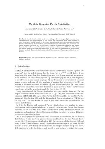
13The GP distribution has the following pdf1f (x) a kx (1 k)/k1 a0 x if k 00 x a/k if k 0(iii) The Weibull distribution with three parameters (TPWD).The density of this distribution is given by x a γf (x) γb γ (x a) γ 1 exp ,x abγ, b 0.(iv) The Beta Pareto distribution (BPD). The density of this distribution ispresented in Equation 6.In order to compare the models we will use the K-S statistic given byKS (Fest ) max Fn (xi ) Fest (xi ) ,(21)1 i nwhere Fest is the model’s c.d.f using the estimated parameters. We will also providethe absolute mean distance statistic given byn1XD (Fest ) Fn (xi ) Fest (xi ) n(22)i 14.1.Castelo RiverThe data consist of 684 maximum values of monthly flood rates of the CasteloRiver, in Brazil, and it is available online (hidroweb.ana.gov.br). Table 1 showssummary statistics of the data. The Figure 3 shows the histogram and box plot ofthe data. It is worth noticing the strong asymmetry of the distribution of the datato the right. This behavior is quite common in hydrology data.Table 1.Descriptive statistics of maximum monthly flood rate of Castelo River.Min.0.7401st Qu.4.602Median6.555Mean7.7043rd Qu.9.678Max.33.4Std. Dev.4.6178The Table 2 and Figure 4 present the results obtained by the MDE. The K-S andD statistics present very high values for TPD and GPD, suggesting a quite pooradjust to the data. Despite this improvement, the KS-statistic remained very high.The K-S test rejected both, TPD and GPD distributions, as appropriate models.For the TPWD, the D and K-S statistics are better than for the TPD and GPD.The K-S test now does not reject the TPWD as an appropriate model at 5% ofsignificance.For the Beta Pareto distribution and BTPD the K-S test does not reject eithermodels, even at 10% of significance. The Figure 4 shows the empirical cdf and fittedcdf for all models.
14REFERENCES(a)(b) 15201000051050Frequency2515030 05101520253035FloodFigure 3. Castelo River flood: (a) Histogram (b) Box-Plot.Table 2.KS Estimative of parameters and KS and D statistics.TPDk̂ 10312 ;GPDâ 12.0612;k̂ Dâ 0.74;b̂ 7.4360;γ̂ 1.8658;0.03990.0207BPDα̂ 15.79;β̂ 64.14;k̂ 0.1;0.02760.0116BTPDα̂ 9.8228;β̂ 3.9035;k̂ 0.347;0.01820.0082ConclusionIn this work a new family of distribution called Beta truncated Pareto distributionwas introduced and some of its properties were analysed. The BTPD proved to bea very flexible model with many different forms for its density (as it can be seen inFigure 1). Also, the BTPD includes some other families that were already proposedin literature. For the parameters estimation we used the minimum distance method.In order to evaluate the BTPD performance we applied the BTPD to real data.The TPD and GPD a very poor fit. The TPWD had a good fit was not rejectedby the KS test. The BTPD and BPD have the best fit to the data with a smalladvantage for BTPD. They both followed the empirical distribution very closelywhen the MDE were applied.Due to the fact that the BTPD has two more paramaters than the TPWD,one could be favorable to TPWD arguing that the difference between the adjustobtained by the TPWD and the adjust obtained by the BTPD is small. That isnot so clear. Despite the KS test does not reject either, we have a sample size of684 which makes the cost of the two additional parameters not so high. Beyondthat the K-S statistic for the BTPD is less than a half of the KS statistic for theTPWD.References[1] B. C. Arnold, Pareto Distribution, Fairland: International Co-operative Publishing House (1983).[2] B. Gutenberg and R. F. Richter, Frequency of earthquakes in california., Bulletin of the SeismologicalSociety of America (1944).[3] E. T. Lu and R. J. Hamilton, Avalanches of the distribution of solar flares., Astrophysical Journal(1991).
ed Pareto vs BTPD1.0Truncated Pareto vs 20253005101520xxThree Parameters Weibull vs BTPDBeta Pareto vs 51015202530xFigure 4. Empirical cdf and fitted cdf for the truncated Pareto, Three Parameter Weibull, GeneralizedPareto, Beta Pareto and BTPD distributions, for the Castelo River Data, using MDM[4] M. S. Wheatland and P. A. Sturrock, Avalanche models of solar flares and the distribution of activeregions., Astrophysical Journal (1991).[5] G. K. Zipf, Human Behaviour and the Principle of Least Effort., Addison-Wesley, Cambridge (1949).[6] D. H. Zanette and S. C. Manrubia, Vertical transmission of culture and the distribution of familynames., Physic A (2001).[7] A. J. Lotka, The frequency distribution of scientific production., J. Wash. Acad. Sci. (1926).[8] D. J. de S. Price, Networks of scientific papers., Science (1965).[9] B. D. Malamud and D. L. Turcotte, The applicability of power-law frequency statistics to floods,Journal of Hydrology (2006).[10] O. S. Klass, O. Biham, M. Levy, O. Malcai and S. Solomon, The Forbes 400 and the Pareto wealthdistribution, Economics Letters (2006).[11] A. Jayadev, A power law tail in India’s wealth distribution: Evidence from survey data, Physic A(2008).[12] S. Sinha, Evidence for power-law tail of the wealth distribution in India, Physic A (2006).[13] R. V. Hogg, J. W. Mckean and A. T. Craig Introduction to Mathematical Statistics, 6th ed. PearsonPrentice-Hall, New Jersey (2005).[14] I. B. Aban, M. M. Meerschaert and A. K. Panorska Paramete Estimation for the truncated ParetoDistribution, Jounal of the American Statistical Association (2006).[15] L. Zaninetti and M. Ferraro On the truncated Pareto distribution with application, Central EuropeanJournal of Physics (2008).[16] W. J. Reed, The Pareto, Zipf and other power laws, Economics Letter (2001).[17] W. J. Reed, The Pareto law of incomes - an explanation and an extension, Physic A (2003).[18] J. R. M. Hosking and J. R. Wallis, Parameter and quantile estimation for the generalized Paretodistribution. Technometrics (1987).[19] S. D. Grimshaw, Computing maximum likelihood estimates for the generalized Pareto distribution.,Technometrics (1993).[20] R. A. Lockhart and M. A. Stephens Estimation and Tests of Fit for the Three-parameter Weibulldistribution, Journal of the Royal Statistical Society. B (1994).[21] J. M. F. Carrasco, E. M. M. Ortega and G. M. Cordeiro A generalized modified Weibull distributionfor lifetime modeling, Computational Statistics and Data Analysis (2008).[22] A. C. Cohen and B. J. Whitten Modified moment and maximum likelihood estimators for parameters
RENCESof the three-parameter gamma distribution, Communications in Statistics - Simulation and Computation (1982).R. D. Gupta and D. Kundu Exponentiated Exponential Family: An Alternative to Gamma and WeibullDistributions, Biometrical Journal (2001).W. Nelson, Applied Life Data Analysis, John Wiley and Sons Inc. (1982), New York.N. Eugene, C. Lee and F. Famoye, B eta-Normal Distributions and Its Applications, Communicationsin Statistics - Theory and Methods (2002), pp. 497–512M. C. Jones, Families of distributions arising from distributions of orders statistics, TEST vol. 13(2004), pp. 1–43.A. Akinsete, F. Famoye and C. Lee, The beta-Pareto distribution, Statistcs (2008), pp. 547–563K. Zografos and N. Balakrishnan, On families of beta- and generalized gamma-generated distributionsand associated inference, Statistical Methodology (2009).M. O. Lorenz Methods for measuring concentration of wealth., Journal of American Statistical Association (1905).M. H. Gail and R. M. Pfeiffer On criteria for evaluating models of absolute risk, Biostatistics (2005).J. Wolfowitz Estimation by the minimum distance method, Ann. Inst. Statist. Math (1953).D. Pollard The minimum distance method of testing, Metrika (1980).A. Luceño Fitting the generalized Pareto distribution to data using maximum goodness-of-fit estimators, Computational Statistics & Data Analysis (2006).
1 The Beta Truncated Pareto Distribution Lourenzutti R. a, Duarte D. , Castellares F. and Azevedo M. Universidade Federal de Minas Gerais,Belo Horizonte, MG, Brazil; The Pareto distribution is widely used to modelling a diverse range of phenomena.