WIXLIB

4Prerequisitesthis relationship by stating that the set C is a subset of the set S, which is written in symbols asC S. The more formal definition is given below.Definition 0.3. Given sets A and B, we say that the set A is a subset of the set B and write‘A B’ if every element in A is also an element of B.Note that in our example above C S, but not vice-versa, since o 2 S but o 2/ C. Additionally,the set of vowels V {a, e, i, o, u}, while it does have an element in common with S, is not asubset of S. (As an added note, S is not a subset of V , either.) We could, however, build a setwhich contains both S and V as subsets by gathering all of the elements in both S and V togetherinto a single set, say U {s, m, o, l, k, a, e, i, u}. Then S U and V U. The set U we havebuilt is called the union of the sets S and V and is denoted S [ V . Furthermore, S and V aren’tcompletely different sets since they both contain the letter ‘o.’ The intersection of two sets is theset of elements (if any) the two sets have in common. In this case, the intersection of S and V is{o}, written S \ V {o}. We formalize these ideas below.Definition 0.4. Suppose A and B are sets. The intersection of A and B is A \ B {x x 2 A and x 2 B} The union of A and B is A [ B {x x 2 A or x 2 B (or both)}The key words in Definition 0.4 to focus on are the conjunctions: ‘intersection’ corresponds to‘and’ meaning the elements have to be in both sets to be in the intersection, whereas ‘union’corresponds to ‘or’ meaning the elements have to be in one set, or the other set (or both). In otherwords, to belong to the union of two sets an element must belong to at least one of them.Returning to the sets C and V above, C [ V {s, m, l, k , a, e, i, o, u}.2 When it comes to theirintersection, however, we run into a bit of notational awkwardness since C and V have no elementsin common. While we could write C \ V {}, this sort of thing happens often enough that we givethe set with no elements a name.Definition 0.5. The Empty Set ; is the set which contains no elements. That is,; {} {x x 6 x}.As promised, the empty set is the set containing no elements since no matter what ‘x’ is, ‘x x.’Like the number ‘0,’ the empty set plays a vital role in mathematics.3 We introduce it here more asa symbol of convenience as opposed to a contrivance.4 Using this new bit of notation, we have forthe sets C and V above that C \ V ;. A nice way to visualize relationships between sets and setoperations is to draw a Venn Diagram. A Venn Diagram for the sets S, C and V is drawn at thetop of the next page.2Which just so happens to be the same set as S [ V .Sadly, the full extent of the empty set’s role will not be explored in this text.4Actually, the empty set can be used to generate numbers - mathematicians can create something from nothing!3

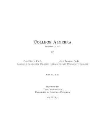
0.1 Basic Set Theory and Interval Notation5UCosmlkaeiuSVA Venn Diagram for C, S and V .In the Venn Diagram above we have three circles - one for each of the sets C, S and V . Wevisualize the area enclosed by each of these circles as the elements of each set. Here, we’vespelled out the elements for definitiveness. Notice that the circle representing the set C is completely inside the circle representing S. This is a geometric way of showing that C S. Also,notice that the circles representing S and V overlap on the letter ‘o’. This common region is howwe visualize S \ V . Notice that since C \ V ;, the circles which represent C and V have nooverlap whatsoever.All of these circles lie in a rectangle labeled U (for ‘universal’ set). A universal set contains allof the elements under discussion, so it could always be taken as the union of all of the sets inquestion, or an even larger set. In this case, we could take U S [ V or U as the set of lettersin the entire alphabet. The reader may well wonder if there is an ultimate universal set whichcontains everything. The short answer is ‘no’ and we refer you once again to Russell’s Paradox.The usual triptych of Venn Diagrams indicating generic sets A and B along with A \ B and A [ Bis given below.UUUA\BABSets A and B.AA[BBA \ B is shaded.ABA [ B is shaded.

6Prerequisites0.1.2Sets of Real NumbersThe playground for most of this text is the set of Real Numbers. Many quantities in the ‘real world’can be quantified using real numbers: the temperature at a given time, the revenue generatedby selling a certain number of products and the maximum population of Sasquatch which caninhabit a particular region are just three basic examples. A succinct, but nonetheless incomplete5definition of a real number is given below.Definition 0.6. A real number is any number which possesses a decimal representation. Theset of real numbers is denoted by the character R.Certain subsets of the real numbers are worthy of note and are listed below. In fact, in moreadvanced texts,6 the real numbers are constructed from some of these subsets.Special Subsets of Real Numbers1. The Natural Numbers: N {1, 2, 3, .} The periods of ellipsis ‘.’ here indicate that thenatural numbers contain 1, 2, 3 ‘and so forth’.2. The Whole Numbers: W {0, 1, 2, .}.3. The Integers: Z {. , 3, 2, 1, 0, 1, 2, 3, .} {0, 1, 2, 3, .}.a4. The Rational Numbers: Q ba a 2 Z and b 2 Z . Rational numbers are the ratios ofintegers where the denominator is not zero. It turns out that another way to describe therational numbersb is:Q {x x possesses a repeating or terminating decimal representation}5. The Irrational Numbers: P {x x 2 R but x 2/ Q}.c That is, an irrational number is areal number which isn’t rational. Said differently,P {x x possesses a decimal representation which neither repeats nor terminates}aThe symbol is read ‘plus or minus’ and it is a shorthand notation which appears throughout the text. Justremember that x 3 means x 3 or x 3.bSee Section 9.2.pcExamples here include number (See Section 10.1), 2 and 0.101001000100001 .Note that every natural number is a whole number which, in turn, is an integer. Each integer is arational number (take b 1 in the above definition for Q) and since every rational number is a realnumber7 the sets N, W, Z, Q, and R are nested like Matryoshka dolls. More formally, these setsform a subset chain: N W Z Q R. The reader is encouraged to sketch a Venn Diagramdepicting R and all of the subsets mentioned above. It is time for an example.5Math pun intended!See, for instance, Landau’s Foundations of Analysis.7Thanks to long division!6

0.1 Basic Set Theory and Interval Notation7Example 0.1.1.1. Write a roster description for P {2n n 2 N} and E {2n n 2 Z}.2. Write a verbal description for S {x 2 x 2 R}.3. Let A { 117, 45 , 0.202002, 0.202002000200002 .}.(a) Which elements of A are natural numbers? Rational numbers? Real numbers?(b) Find A \ W, A \ Z and A \ P.4. What is another name for N [ Q? What about Q [ P?Solution.1. To find a roster description for these sets, we need to list their elements. Starting withP {2n n 2 N}, we substitute natural number values n into the formula 2n . For n 1 we get21 2, for n 2 we get 22 4, for n 3 we get 23 8 and for n 4 we get 24 16. Hence Pdescribes the powers of 2, so a roster description for P is P {2, 4, 8, 16, .} where the ‘.’indicates the that pattern continues.8Proceeding in the same way, we generate elements in E {2n n 2 Z} by plugging in integervalues of n into the formula 2n. Starting with n 0 we obtain 2(0) 0. For n 1 we get2(1) 2, for n 1 we get 2( 1) 2 for n 2, we get 2(2) 4 and for n 2 we get2( 2) 4. As n moves through the integers, 2n produces all of the even integers.9 A rosterdescription for E is E {0, 2, 4, .}.2. One way to verbally describe S is to say that S is the ‘set of all squares of real numbers’.While this isn’t incorrect, we’d like to take this opportunity to delve a little deeper.10 Whatmakes the set S {x 2 x 2 R} a little trickier to wrangle than the sets P or E above is thatthe dummy variable here, x, runs through all real numbers. Unlike the natural numbers orthe integers, the real numbers cannot be listed in any methodical way.11 Nevertheless, wecan select some real numbers, square them and get a sense of what kind of numbers lie inp2S. For x 2, x 2 ( 2)2 4 so 4 is in S, as are 23 94 and ( 117)2 117. Even thingslike ( )2 and (0.101001000100001 .)2 are in S.So suppose s 2 S. What can be said about s? We know there is some real number x sothat s x 2 . Since x 2 0 for any real number x, we know s 0. This tells us that everything8This isn’t the most precise way to describe this set - it’s always dangerous to use ‘.’ since we assume that thepattern is clearly demonstrated and thus made evident to the reader. Formulas are more precise because the patternis clear.9This shouldn’t be too surprising, since an even integer is defined to be an integer multiple of 2.10Think of this as an opportunity to stop and smell the mathematical roses.11This is a nontrivial statement. Interested readers are directed to a discussion of Cantor’s Diagonal Argument.

8Prerequisitesin S is a non-negative real number.12 This begs the question: are all of the non-negativereal numbers in S? Suppose n is a non-negative real number, that is, n 0. If n were in S,2 n bythere would be a real number xpso that x 2 n. pAs you may recall, we can solve xp‘extracting square roots’: x n. Since n 0, n is a real number.13 Moreover, ( n)2 nso n is the square of a real number which means n 2 S. Hence, S is the set of non-negativereal numbers.3. (a) The set A contains no natural numbers.14 Clearly, 45 is a rational number as is 117(which can be written as 1171 ). It’s the last two numbers listed in A, 0.202002 and0.202002000200002 ., that warrant some discussion. First, recall that the ‘line’ overthe digits 2002 in 0.202002 (called the vinculum) indicates that these digits repeat, so itis a rational number.15 As for the number 0.202002000200002 ., the ‘.’ indicates thepattern of adding an extra ‘0’ followed by a ‘2’ is what defines this real number. Despitethe fact there is a pattern to this decimal, this decimal is not repeating, so it is not arational number - it is, in fact, an irrational number. All of the elements of A are realnumbers, since all of them can be expressed as decimals (remember that 45 0.8).(b) The set A \ W {x x 2 A and x 2 W} is another way of saying we are looking forthe set of numbers in A which are whole numbers. Since A contains no whole numbers, A \ W ;. Similarly, A \ Z is looking for the set of numbers in A which areintegers. Since 117 is the only integer in A, A \ Z { 117}. As for the set A \ P,as discussed in part (a), the number 0.202002000200002 . is irrational, so A \ P {0.202002000200002 .}.4. The set N [ Q {x x 2 N or x 2 Q} is the union of the set of natural numbers with the setof rational numbers. Since every natural number is a rational number, N doesn’t contributeany new elements to Q, so N [ Q Q.16 For the set Q [ P, we note that every real numberis either rational or not, hence Q [ P R, pretty much by the definition of the set P.As you may recall, we often visualize the set of real numbers R as a line where each point on theline corresponds to one and only one real number. Given two different real numbers a and b, wewrite a b if a is located to the left of b on the number line, as shown below.abThe real number line with two numbers a and b where a b.While this notion seems innocuous, it is worth pointing out that this convention is rooted in twodeep properties of real numbers. The first property is that R is complete. This means that there12This means S is a subset of the non-negative real numbers.This is called the ‘square root closed’ property of the non-negative real numbers.14Carl was tempted to include 0.9 in the set A, but thought better of it. See Section 9.2 for details.15So 0.202002 0.20200220022002 .16In fact, anytime A B, A [ B B and vice-versa. See the exercises.13

0.1 Basic Set Theory and Interval Notation9are no ‘holes’ or ‘gaps’ in the real number line.17 Another way to think about this is that if youchoose any two distinct (different) real numbers, and look between them, you’ll find a solid linesegment (or interval) consisting of infinitely many real numbers. The next result tells us what typesof numbers we can expect to find.Density Property of Q and P in RBetween any two distinct real numbers, there is at least one rational number and irrationalnumber. It then follows that between any two distinct real numbers there will be infinitely manyrational and irrational numbers.The root word ‘dense’ here communicates the idea that rationals and irrationals are ‘thoroughlymixed’ into R. The reader is encouraged to think about how one would find both a rational and anirrational number between, say, 0.9999 and 1. Once you’ve done that, try doing the same thing forthe numbers 0.9 and 1. (‘Try’ is the operative word, here.18 )The second property R possesses that lets us view it as a line is that the set is totally ordered.This means that given any two real numbers a and b, either a b, a b or a b which allowsus to arrange the numbers from least (left) to greatest (right). You may have heard this propertygiven as the ‘Law of Trichotomy’.Law of TrichotomyIf a and b are real numbers then exactly one of the following statements is true:a ba ba bSegments of the real number line are called intervals. They play a huge role not only in thistext but also in the Calculus curriculum so we need a concise way to describe them. We start byexamining a few examples of the interval notation associated with some specific sets of numbers.Set of Real NumbersInterval Notation{x 1 x 3}[1, 3){x 1 x 4}{x x 5}{x x 2}[ 1, 4]Region on the Real Number Line131( 1, 5]( 2, 1)452As you can glean from the table, for intervals with finite endpoints we start by writing ‘left endpoint,right endpoint’. We use square brackets, ‘[’ or ‘]’, if the endpoint is included in the interval. This17Alas, this intuitive feel for what it means to be ‘complete’ is as good as it gets at this level. Completeness does geta much more precise meaning later in courses like Analysis and Topology.18Again, see Section 9.2 for details.

10Prerequisitescorresponds to a ‘filled-in’ or ‘closed’ dot on the number line to indicate that the number is includedin the set. Otherwise, we use parentheses, ‘(’ or ‘)’ that correspond to an ‘open’ circle whichindicates that the endpoint is not part of the set. If the interval does not have finite endpoints, weuse the symbol 1 to indicate that the interval extends indefinitely to the left and the symbol 1to indicate that the interval extends indefinitely to the right. Since infinity is a concept, and not anumber, we always use parentheses when using these symbols in interval notation, and use theappropriate arrow to indicate that the interval extends indefinitely in one or both directions. Wesummarize all of the possible cases in one convenient table below.19Interval NotationLet a and b be real numbers with a b.Set of Real NumbersInterval Notation{x a x b}(a, b)ab{x a x b}[a, b)ab{x a x b}(a, b]ab{x a x b}[a, b]ab{x x b}( 1, b)b{x x b}( 1, b]b{x x a}(a, 1)a{x x[a, 1)aRa}Region on the Real Number Line( 1, 1)We close this section with an example that ties together several concepts presented earlier. Specifically, we demonstrate how to use interval notation along with the concepts of ‘union’ and ‘intersection’ to describe a variety of sets on the real number line.19The importance of understanding interval notation in Calculus cannot be overstated so please do yourself a favorand memorize this chart.

0.1 Basic Set Theory and Interval Notation11Example 0.1.2.1. Express the following sets of numbers using interval notation.(a) {x x 2 or x(c) {x x 6 3}2}(b) {x x 6 3}(d) {x 1 x 3 or x 5}2. Let A [ 5, 3) and B (1, 1). Find A \ B and A [ B.Solution.1. (a) The best way to proceed here is to graph the set of numbers on the number lineand glean the answer from it. The inequality x 2 corresponds to the interval( 1, 2] and the inequality x2 corresponds to the interval [2, 1). The ‘or’ in{x x 2 or x2} tells us that we are looking for the union of these two intervals,so our answer is ( 1, 2] [ [2, 1).22( 1, 2] [ [2, 1)(b) For the set {x x 6 3}, we shade the entire real number line except x 3, where weleave an open circle. This divides the real number line into two intervals, ( 1, 3) and(3, 1). Since the values of x could be in one of these intervals or the other, we onceagain use the union symbol to get {x x 6 3} ( 1, 3) [ (3, 1).3( 1, 3) [ (3, 1)(c) For the set {x x 6 3}, we proceed as before and exclude both x 3 and x 3 fromour set. (Do you remember what we said back on 6 about x 3?) This breaks thenumber line into three intervals, ( 1, 3), ( 3, 3) and (3, 1). Since the set describesreal numbers which come from the first, second or third interval, we have {x x 6 3} ( 1, 3) [ ( 3, 3) [ (3, 1).33( 1, 3) [ ( 3, 3) [ (3, 1)(d) Graphing the set {x 1 x 3 or x 5} yields the interval ( 1, 3] along with thesingle number 5. While we could express this single point as [5, 5], it is customary towrite a single point as a ‘singleton set’, so in our case we have the set {5}. Thus ourfinal answer is {x 1 x 3 or x 5} ( 1, 3] [ {5}.13 5( 1, 3] [ {5}

12Prerequisites2. We start by graphing A [ 5, 3) and B (1, 1) on the number line. To find A\B, we need tofind the numbers in common to both A and B, in other words, the overlap of the two intervals.Clearly, everything between 1 and 3 is in both A and B. However, since 1 is in A but not inB, 1 is not in the intersection. Similarly, since 3 is in B but not in A, it isn’t in the intersectioneither. Hence, A \ B (1, 3). To find A [ B, we need to find the numbers in at least one ofA or B. Graphically, we shade A and B along with it. Notice here that even though 1 isn’tin B, it is in A, so it’s the union along with all the other elements of A between 5 and 1. Asimilar argument goes for the inclusion of 3 in the union. The result of shading both A and Btogether gives us A [ B [ 5, 1).51 3A [ 5, 3), B (1, 1)51 3A \ B (1, 3)51 3A [ B [ 5, 1)

0.1 Basic Set Theory and Interval Notation0.1.313Exercises1. Find a verbal description for O {2n1 n 2 N}2. Find a roster description for X {z 2 z 2 Z} p3203. Let A 3, 1.02,, 0.57, 1.23, 3, 5.2020020002 . , , 1175

College Algebra Version bˇc 3 by Carl Stitz, Ph.D. Jeff Zeager, Ph.D. Lakeland Community College Lorain County Community College July 15, 2011 Modified By Teri Christiansen . Algebra text. An outline of the chapter is given below. Section 0.1 (Basic Set Theory and Interval Notation) contains a brief summary of the set theory .