WIXLIB

1.2. THE VERTEX COVER PROBLEM3solution too much, then we have an efficient approximation algorithm for ourproblem. Approximation Algorithms via Linear Programming. We will give various examples inwhich approximation algorithms can be designed by “rounding” the fractional optimaof linear programs. Exact Algorithms for Flows and Matchings. We will study some of the most elegantand useful optimization algorithms, those that find optimal solutions to “flow” and“matching” problems. Linear Programming, Flows and Matchings. We will show that flow and matchingproblems can be solved optimally via linear programming. Understanding why willmake us give a second look at the theory of linear programming duality. Online Algorithms. An online algorithm is an algorithm that receives its input as astream, and, at any given time, it has to make decisions only based on the partialamount of data seen so far. We will study two typical online settings: paging (and,in general, data transfer in hierarchical memories) and investing.1.21.2.1The Vertex Cover ProblemDefinitionsGiven an undirected graph G (V, E), a vertex cover is a subset of vertices C V suchthat for every edge (u, v) E at least one of u or v is an element of C.In the minimum vertex cover problem, we are given in input a graph and the goal is to finda vertex cover containing as few vertices as possible.The minimum vertex cover problem is very related to the maximum independent set problem. In a graph G (V, E) an independent set is a subset I V of vertices such thatthere is no edge (u, v) E having both endpoints u and v contained in I. In the maximumindependent set problem the goal is to find a largest possible independent set.It is easy to see that, in a graph G (V, E), a set C V is a vertex cover if and only if itscomplement V C is an independent set, and so, from the point of view of exact solutions,the two problems are equivalent: if C is an optimal vertex cover for the graph G then V Cis an optimal independent set for G, and if I is an optimal independent set then V I isan optimal vertex cover.From the point of view of approximation, however, the two problems are not equivalent. Weare going to describe a linear time 2-approximate algorithm for minimum vertex cover, thatis an algorithm that finds a vertex cover of size at most twice the optimal size. It is known,however, that no constant-factor, polynomial-time, approximation algorithms can exist forthe independent set problem. To see why there is no contradiction (and how the notionof approximation is highly dependent on the cost function), suppose that we have a graphwith n vertices in which the optimal vertex cover has size .9 · n, and that our algorithm

4LECTURE 1. INTRODUCTIONfinds a vertex cover of size n 1. Then the algorithm finds a solution that is only about11% larger than the optimum, which is not bad. From the point of view of independent setsize, however, we have a graph in which the optimum independent set has size n/10, andour algorithm only finds an independent set of size 1, which is terrible1.2.2The AlgorithmThe algorithm is very simple, although not entirely natural: Input: graph G (V, E) C : while there is an edge (u, v) E such that u 6 C and v 6 C– C : C {u, v} return CWe initialize our set to the empty set, and, while it fails to be a vertex cover because someedge is uncovered, we add both endpoints of the edge to the set. By the time we are finishedwith the while loop, C is such that for every edge (u, v) E, either u C or v C (orboth), that is, C is a vertex cover.To analyze the approximation, let opt be the number of vertices in a minimal vertex cover,then we observe that If M E is a matching, that is, a set of edges that have no endpoint in common, thenwe must have opt M , because every edge in M must be covered using a distinctvertex. The set of edges that are considered inside the while loop form a matching, because if(u, v) and (u0 , v 0 ) are two edges considered in the while loop, and (u, v) is the one thatis considered first, then the set C contains u and v when (u0 , v 0 ) is being considered,and hence u, v, u0 , v 0 are all distinct. If we let M denote the set of edges considered in the while cycle of the algorithm, andwe let Cout be the set given in output by the algorithm, then we have Cout 2 · M 2 · optAs we said before, there is something a bit unnatural about the algorithm. Every time wefind an edge (u, v) that violates the condition that C is a vertex cover, we add both verticesu and v to C, even though adding just one of them would suffice to cover the edge (u, v).Isn’t it an overkill?Consider the following alternative algorithm that adds only one vertex at a time:

1.2. THE VERTEX COVER PROBLEM5 Input: graph G (V, E) C : while there is an edge (u, v) E such that u 6 C and v 6 C– C : C {u} return CThis is a problem if our graph is a “star.” Then the optimum is to pick the center, whilethe above algorithm might, in the worse case, pick all the vertices except the center.Another alternative would be a greedy algorithm: Input: graph G (V, E) C : while C is not a vertex cover– let u be the vertex incident on the most uncovered edges– C : C {u} return CThe above greedy algorithm also works rather poorly. For every n, we can construct an nvertex graph where the optimum is roughly n/ ln n, but the algorithm finds a solution ofcost roughly n n/ ln n, so that it does not achieve a constant-factor approximation of theoptimum. We will return to this greedy approach and to these bad examples when we talkabout the minimum set cover problem.

6LECTURE 1. INTRODUCTION

Lecture 2Steiner Tree ApproximationIn which we define the Steiner Tree problem, we show the equivalence of metric and generalSteiner tree, and we give a 2-approximate algorithm for both problems.2.1Approximating the Metric Steiner Tree ProblemThe Metric Steiner Tree Problem is defined as follows: the input is a set X R S of points,where R is a set of required points and S is a set of optional points, and a symmetric distancefunction d : X X R 0 that associates a non-negative distance d(x, y) d(y, x) 0 toevery pair of points. We restrict the problem to the case in which d satisfies the triangleinequality, that is, x, y, z X.d(x, z) d(x, y) d(y, z)In such a case, d is called a (semi-)metric, hence the name of the problem.The goal is to find a tree T (V, E), where V is any set R V X of points that includesall of the required points, and possibly some of the optional points, such that the costXcostd (T ) : d(u, v)(u,v) Eof the tree is minimized.This problem is very similar to the minimum spanning tree problem, which we know to havean exact algorithm that runs in polynomial (in fact, nearly linear) time. In the minimumspanning tree problem, we are given a weighted graph, which we can think of as a set ofpoints together with a distance function (which might not satisfy the triangle inequality),and we want to find the tree of minimal total length that spans all the vertices. Thedifference is that in the minimum Steiner tree problem we only require to span a subset of7

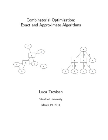
8LECTURE 2. STEINER TREE APPROXIMATIONvertices, and other vertices are included only if they are beneficial to constructing a tree oflower total length.We consider the following very simple approximation algorithm: run a minimum spanningtree algorithm on the set of required vertices, that is, find the best possible tree that usesnone of the optional vertices.We claim that this algorithm is 2-approximate, that is, it finds a solution whose cost is atmost twice the optimal cost.To do so, we prove the following.Lemma 2.1 Let (X R S, d) be an instance of the metric Steiner tree problem, andT (V, E) be a Steiner tree with R V X.Then there is a tree T 0 (R, E 0 ) which spans the vertices in R and only the vertices in Rsuch thatcostd (T 0 ) 2 · costd (T )In particular, applying the Lemma to the optimal Steiner tree we see that there is a spanningtree of R whose cost is at most twice the cost of the optimal Steiner tree. This also meansthat the minimal spanning tree of R also has cost at most twice the cost of the optimalSteiner tree.Proof: [Of Lemma 2.1] Consider a DFS traversal of T , that is, a sequencex0 , x1 , x2 , . . . , xm x0listing the vertices of T in the order in which they are considered during a DFS, includingeach time we return to a vertex at the end of eachPrecursive call. The sequence describesa cycle over the elements of V whose total length mi 0 d(xi , xi 1 ) is precisely 2 · costd (T ),because the cycle uses each edge of the tree precisely twice.Let now y0 , y1 , . . . , yk be the sequence obtained from x0 , . . . , xm by removing the verticesin S and keeping only the first occurrent of each vertex in R.ThenPy0 , . . . , yk is a path that includes all the vertices of R, and no other vertex, and itscost ki 0 d(yi , yi 1 ) is at most the cost of the cycle x0 , x1 , x2 , . . . , xm (here we are usingthe triangle inequality), and so it is at most 2 · costd (T ).But now note that y0 , . . . , yk , being a path, is also a tree, and so we can take T 0 to be tree(R, E 0 ) where E 0 is the edge set {(yi , yi 1 )}i 0,.,k . For example, if we have an instance in which R {a, b, c, d, e, f }, S {g, h}, and thedistance function d(·, ·) assigns distance 1 to the points connected by an edge in the graphbelow, and distance 2 otherwise

2.1. APPROXIMATING THE METRIC STEINER TREE PROBLEM9Then the following is a Steiner tree for our input whose cost is 8:We use the argument in the proof of the Lemma to show that there is a Spanning tree ofR of cost at most 16. (In fact we will do better.)The order in which we visit vertices in a DFS of T is a g d g f g a h c h b h a e a. If we consider it as a loop that starts at a and goesback to a after touching all vertices, some vertices more than once, then the loop has cost16, because it uses every edge exactly twice.Now we note that if we take the DFS traversal, and we skip all the optional vertices and allthe vertices previously visited, we obtain an order in which to visit all the required vertices,and no other vertex. In the example the order is a d f c b e.Because this path was obtained by “shortcutting” a path of cost at most twice the cost ofT , and because we have the triangle inequality, the path that we find has also cost at most

10LECTURE 2. STEINER TREE APPROXIMATIONtwice that of T . In our example, the cost is just 10. Since a path is, in particular, a tree,we have found a spanning tree of R whose cost is at most twice the cost of T .The factor of 2 in the lemma cannot be improved, because there are instances of the MetricSteiner Tree problem in which the cost of the minimum spanning tree of R is, in fact,arbitrarily close to twice the cost of the minimum steiner tree.Consider an instance in which S {v0 }, R {v1 , . . . , vn }, d(v0 , vi ) 1 for i 1, . . . , n,and d(vi , vj ) 2 for all 1 i j n. That is, consider an instance in which the requiredpoints are all at distance two from each other, but they are all at distance one from theunique optional point. Then the minimum Steiner tree has v0 as a root and the nodesv1 , . . . , vn as leaves, and it has cost n, but the minimum spanning tree of R has cost 2n 2,because it is a tree with n nodes and n 1 edges, and each edge is of cost 2.2.2Metric versus General Steiner TreeThe General Steiner Tree problem is like the Metric Steiner Tree problem, but we allowarbitrary distance functions.In this case, it is not true any more that a minimum spanning tree of R gives a goodapproximation: consider the case in which R {a, b}, S {c}, d(a, b) 10100 , d(a, c) 1and d(b, c) 1. Then the minimum spanning tree of R has cost 10100 while the minimumSteiner tree has cost 2.We can show, however, that our 2-approximation algorithm for Metric Steiner Tree can beturned, with some care, into a 2-approximation algorithm for General Steiner Tree.Lemma 2.2 For every c 1, if there is a polynomial time c-approximate algorithm forMetric Steiner Tree, then there is a polynomial time c-approximate algorithm for GeneralSteiner Tree.Proof: Suppose that we have a polynomial-time c-approximate algorithm A for MetricSteiner Tree and that we are given in input an instance (X R S, d) of General SteinerTree. We show how to find, in polynomial time, a c-approximate solution for (X, d).For every two points x, y X, let d0 (x, y) be the length of a shortest path from x to y inthe weighted graph of vertex set X of weights d(·, ·). Note that d0 (·, ·) is a distance functionthat satisfies the triangle inequality, because for every three points x, y, z it must be thecase that the length of the shortest path from x to z cannot be any more than the lengthof the shortest path from x to y plus the length of the shortest path from y to z.This means that (X, d0 ) is an instance of Metric Steiner Tree, and we can apply algorithmA to it, and find a tree T 0 (V 0 , E) of costcostd0 (T 0 ) c · opt(X, d0 )Now notice that, for every pair of points, d0 (x, y) d(x, y), and so if T is the optimal treeof our original input (X, d) we have

2.2. METRIC VERSUS GENERAL STEINER TREE11opt(X, d0 ) costd0 (T ) costd (T ) opt(X, d)So putting all together we havecostd0 (T 0 ) c · opt(X, d)Now, from T 0 , construct a graph G (V, E) by replacing each edge (x, y) by the shortestpath from x to y according to d(·). By our construction we havecostd (G) Xd(x, y) (x,y) EXd0 (x, y) costd0 (T 0 )(x,y) E 0Note also that G is a connected graph.The reason why we have an inequality instead of an equality is that certain edges of G mightbelong to more than one shortest path, so they are counted only once on the left-hand side.Finally, take a minimum spanning tree T of G according to the weights d(·, ·). Now T is avalid Steiner tree, and we havecostd (T ) costd (G) c · opt(X, d)

12LECTURE 2. STEINER TREE APPROXIMATION

Lecture 3TSP and Eulerian CyclesIn which we prove the equivalence of three versions of the Traveling Salesman Problem, weprovide a 2-approximate algorithm, we review the notion of Eulerian cycle, we think of theTSP as the problem of finding a minimum-cost connected Eulerian graph, and we revisit the2-approximate algorithm from this perspective.3.1The Traveling Salesman ProblemIn the Traveling Salesman Problem (abbreviated TSP) we are given a set of points X anda symmetric distance function d : X X R 0 . The goal is to find a cycle that reachesall points in X and whose total length is as short as possible.For example, a shuttle driver that picks up seven people at SFO and needs to take themto their home and then go back to the airport faces a TSP instance in which X includeseight points (the seven home addresses and the airport), and the distance function is thedriving time between two places. A DHL van driver who has to make a series of deliveryand then go back to the warehouse has a similar problem. Indeed TSP is a basic model forseveral concrete problems, and it one of the most well studied problems in combinatorialoptimization.There are different versions of this problem depending on whether we require d(·, ·) to satisfythe triangle inequality or not, and whether we allow the loop to pass through the same pointmore than once.1. General TSP without repetitions (General TSP-NR): we allow arbitrary symmetricdistance functions, and we require the solution to be a cycle that contains every pointexactly once;2. General TSP with repetitions (General TSP-R): we allow arbitrary symmetric distancefunctions, and we allow all cycles as an admissible solution, even those that containsome point more than once;13

14LECTURE 3. TSP AND EULERIAN CYCLES3. Metric TSP without repetitions (Metric TSP-NR): we only allow inputs in which thedistance function d(·, ·) satisfies the triangle inequality, that is x, y, z X. d(x, z) d(x, y) d(y, z)and we only allow solutions in which each point is reached exactly once;4. Metric TSP with repetitions (Metric TSP-R): we only allow inputs in which the distance function satisfies the triangle inequality, and we allow all cycles as admissiblesolutions, even those that contain some point more than once.For all versions, it is NP-hard to find an optimal solution.If we allow arbitrary distance functions, and we require the solution to be a cycle thatreaches every point exactly once, then we have a problem for which no kind of efficientapproximation is possible.Fact 3.1 If P 6 NP then there is no polynomial-time constant-factor approximation algorithm for General TSP-NR.More generally, if there is a function r : N N such that r(n) can be computable in time2polynomial in n (for example, r(n) 2100 · 2n ), and a polynomial time algorithm that, oninput an instance (X, d) of General TSP-NR with n points finds a solution of cost at mostr(n) times the optimum, then P NP.The other three versions, however, are completely equivalent from the point of view ofapproximation and, as we will see, can be efficiently approximated reasonably well.Lemma 3.2 For every c 1, there is a polynomial time c-approximate algorithm for MetricTSP-NR if and only if there is a polynomial time c-approximate approximation algorithmfor Metric TSP-R. In particular:1. If (X, d) is a Metric TSP input, then the cost of the optimum is the same whether ornot we allow repetitions.2. Every c-approximate algorithm for Metric TSP-NR is also a c-approximate algorithmfor Metric TSP-R.3. Every c-approximate algorithm for Metric TSP-R can be turned into a c-approximatealgorithm for Metric TSP-NR after adding a linear-time post-processing step.Proof: Let optT SP R (X, d) be the cost of an optimal solution for (X, d) among all solutionswith or without repetitions, and optT SP N R (X, d) be the cost of an optimal solution for(X, d) among all solutions without repetitions. Then clearly in the former case we areminimizing over a larger set of possible solutions, and so

3.1. THE TRAVELING SALESMAN PROBLEM15optT SP R (X, d) optT SP N R (X, d)Consider now any cycle, possibly with repetitions, C v0 v1 v2 · · · vm 1 vm v0 . Create a new cycle C 0 from C by removing from C all the repeated occurrences of anyvertex. (With the special case of v0 which is repeated at the end.) For example, the cycleC a c b a d b a becomes a c b d a. Because of the triangleinequality, the total length of C 0 is at most the total length of C, and C 0 is a cycle with norepetitions. If we apply the above process by taking C to be the optimal solution of (X, d)allowing repetitions, we see thatoptT SP R (X, d) optT SP N R (X, d)and so we have proved our first claim that optT SP R (X, d) optT SP N R (X, d).Regarding the second claim, suppose that we have a c-approximate algorithm for MetricTSP-NR. Then, given an input (X, d) the algorithm finds a cycle C with no repetitionssuch thatcostd (C) c · optT SP N R (X, d)but C is also an admissible solution for the problem Metric TSP-R, andcostd (C) c · optT SP N R (X, d) c · optT SP R (X, d)and so our algorithm is also a c-approximate algorithm for optT SP N R .To prove the third claim, suppose we have a c-approximate algorithm for Metric TSP-R.Then, given an input (X, d) the algorithm finds a cycle C, possibly with repetitions, suchthatcostd (C) c · optT SP R (X, d)Now, convert C to a solution C 0 that has no repetitions and such that costd (C 0 ) costd (C)as described above, and output the solution C 0 . We have just described a c-approximatealgorithm for Me

Lecture 1 Introduction In which we describe what this course is about and give a simple example of an approximation algorithm 1.1 Overview In this course we study algorithms for combinatorial optimization problems.