WIXLIB

7.1.37.1.47.1.57.1.6Case III: Repeated Eigenvalues . . . . . . . . . . . . . . . . . . . . . . . . . . . . . . . . .Case IV: Complex Eigenvalues . . . . . . . . . . . . . . . . . . . . . . . . . . . . . . . . . .Case V: Pure Imaginary Eigenvalues . . . . . . . . . . . . . . . . . . . . . . . . . . . . .Summary and Observations . . . . . . . . . . . . . . . . . . . . . . . . . . . . . . . . . . . .1691701701727.2Autonomous Systems and Stability1727.2.1Stability and Instability . . . . . . . . . . . . . . . . . . . . . . . . . . . . . . . . . . . . . . . . . 1737.3Locally Linear Systems7.3.17.3.2Introduction to Nonlinear Systems . . . . . . . . . . . . . . . . . . . . . . . . . . . . . . . 174Linearization around Critical Points . . . . . . . . . . . . . . . . . . . . . . . . . . . . . . 1747.4Predator-Prey Equations174176Partial Differential EquationsVI8Introduction to Partial Differential Equations . . . . . . . . . . . 1838.1Two-Point Boundary Value Problems and Eigenfunctions8.1.18.1.2Boundary Conditions . . . . . . . . . . . . . . . . . . . . . . . . . . . . . . . . . . . . . . . . . . 183Eigenvalue Problems . . . . . . . . . . . . . . . . . . . . . . . . . . . . . . . . . . . . . . . . . . 1858.2Fourier Series8.2.1The Euler-Fourier Formula . . . . . . . . . . . . . . . . . . . . . . . . . . . . . . . . . . . . . . . 1888.3Convergence of Fourier Series8.3.1Convergence of Fourier Series . . . . . . . . . . . . . . . . . . . . . . . . . . . . . . . . . . 1948.4Even and Odd Functions8.4.18.4.2Fourier Sine Series . . . . . . . . . . . . . . . . . . . . . . . . . . . . . . . . . . . . . . . . . . . . . 197Fourier Cosine Series . . . . . . . . . . . . . . . . . . . . . . . . . . . . . . . . . . . . . . . . . . . 1998.5The Heat Equation8.5.1Derivation of the Heat Equation . . . . . . . . . . . . . . . . . . . . . . . . . . . . . . . . . 2028.6Separation of Variables and Heat Equation IVPs2038.6.18.6.28.6.38.6.4Initial Value Problems . . . . . . . . . . . . . . . . . . . . . . . . . . . . . . . . . . . . . . . . . .Separation of Variables . . . . . . . . . . . . . . . . . . . . . . . . . . . . . . . . . . . . . . . .Neumann Boundary Conditions . . . . . . . . . . . . . . . . . . . . . . . . . . . . . . . . .Other Boundary Conditions . . . . . . . . . . . . . . . . . . . . . . . . . . . . . . . . . . . . .2032042072088.7Heat Equation Problems2088.7.1Examples . . . . . . . . . . . . . . . . . . . . . . . . . . . . . . . . . . . . . . . . . . . . . . . . . . . . 2108.8Other Boundary Conditions8.8.18.8.28.8.3Mixed Homogeneous Boundary Conditions . . . . . . . . . . . . . . . . . . . . . . . 212Nonhomogeneous Dirichlet Conditions . . . . . . . . . . . . . . . . . . . . . . . . . . 213Other Boundary Conditions . . . . . . . . . . . . . . . . . . . . . . . . . . . . . . . . . . . . . 2168.9The Wave Equation8.9.18.9.28.9.3Derivation of the Wave Equation . . . . . . . . . . . . . . . . . . . . . . . . . . . . . . . . 216The Homogeneous Dirichlet Problem . . . . . . . . . . . . . . . . . . . . . . . . . . . . 218Examples . . . . . . . . . . . . . . . . . . . . . . . . . . . . . . . . . . . . . . . . . . . . . . . . . . . . 219183187192196201212216

8.10Laplace’s Equation2218.10.18.10.28.10.38.10.4Dirichlet Problem for a Rectangle . . . . . . . . . . . . . . . . . . . . . . . . . . . . . . .Dirichlet Problem For A Circle . . . . . . . . . . . . . . . . . . . . . . . . . . . . . . . . . . .Example 1 . . . . . . . . . . . . . . . . . . . . . . . . . . . . . . . . . . . . . . . . . . . . . . . . . . .Example 2 . . . . . . . . . . . . . . . . . . . . . . . . . . . . . . . . . . . . . . . . . . . . . . . . . . .221222224225

IClassification of DifferentialEquations1Introduction . . . . . . . . . . . . . . . . . . . . . . 111.11.2IntroductionSome Basic Mathematical Models; DirectionFieldsSolutions of Some Differential EquationsClassifications of Differential Equations1.31.4

1. Introduction1.1IntroductionThis set of lecture notes was built from a one semester course on the Introduction toOrdinary and Differential Equations at Penn State University from 2010-2014. Our mainfocus is to develop mathematical intuition for solving real world problems while developingour tool box of useful methods. Topics in this course are derived from five principle subjectsin Mathematics(i) First Order Equations (Ch. 2)(ii) Second Order Linear Equations (Ch. 3)(iii) Higher Order Linear Equations (Ch. 4)(iv) Laplace Transforms (Ch. 5)(v) Systems of Linear Equations (Ch. 6)(vi) Nonlinear Differential Equations and Stability (Ch. 7)(vii) Partial Differential Equations and Fourier Series (Ch. 8)Each class individually goes deeper into the subject, but we will cover the basic toolsneeded to handle problems arising in physics, materials sciences, and the life sciences.Here we focus on the development of the solution methods for solving those problems.1.2Some Basic Mathematical Models; Direction Fields

Chapter 1. Introduction12Definition 1.2.1 A differential equation is an equation containing derivatives.Definition 1.2.2 A differential equation that describes some physical process is oftencalled a mathematical model Example 1.1 (Falling Object)γv( )mgConsider an object falling from the sky. From Newton’s Second Law we haveF ma mdvdt(1.1)When we consider the forces from the free body diagram we also haveF mg γv(1.2)where γ is the drag coefficient. Combining the twomdv mg γvdt(1.3)Suppose m 10kg and γ 2kg/s. Then we havedvv 9.8 dt5(1.4)It looks like the direction field tends towards v 49m/s. We plot the direction field byplugging in the values for v and t and letting dv/dt be the slope of a line at that point. Direction Fields are valuable tools in studying the solutions of differential equations ofthe formdy f (t, y)dt(1.5)where f is a given function of the two variables t and y, sometimes referred to as a ratefunction. At each point on the grid, a short line is drawn whose slope is the value of f atthe point. This technique provides a good picture of the overall behavior of a solution.Two Things to keep in mind:

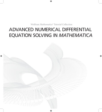
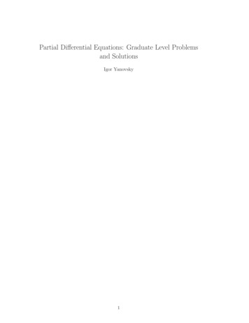
1.2 Some Basic Mathematical Models; Direction Fields13Figure 1.1: Direction field for above example1. In constructing a direction field we never have to solve the differential equation onlyevaluate it at points.2. This method is useful if one has access to a computer because a computer can generatethe plots well. Example 1.2 (Population Growth) Consider a population of field mice, assuming thereis nothing to eat the field mice, the population will grow at a constant rate. Denote time byt (in months) and the mouse population by p(t), then we can express the model asdp rpdt(1.6)where the proportionality factor r is called the rate constant or growth constant. Nowsuppose owls are killing mice (15 per day), the model becomesdp 0.5p 450dt(1.7)note that we subtract 450 rather than 15 because time was measured in months. In generaldp rp kdt(1.8)where the growth rate is r and the predation rate k is unspecified. Note the equilibriumsolution would be k/r.Definition 1.2.3 The equilibrium solution is the value of p(t) where the system nolonger changes,dpdt 0.In this example solutions above equilibrium will increase, while solutions below willdecrease. Steps to Constructing Mathematical Models:1. Identify the independent and dependent variables and assign letters to represent them.

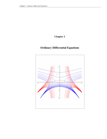
Chapter 1. Introduction14Figure 1.2: Direction field for above exampleOften the independent variable is time.2. Choose the units of measurement for each variable.3. Articulate the basic principle involved in the problem.4. Express the principle in the variables chosen above.5. Make sure each term has the same physical units.6. We will be dealing with models in this chapter which are single differential equations. Example 1.3 Draw the direction field for the following, describe the behavior of y ast . Describe the dependence on the initial value:y0 2y 3(1.9)Ans: For y 1.5 the slopes are positive, and hence the solutions increase. For y 1.5the slopes are negative, and hence the solutions decrease. All solutions appear to divergeaway from the equilibrium solution y(t) 1.5. Example 1.4 Write down a DE of the form dy/dt ay b whose solutions have therequired behavior as t . It must approach 23 .Answer: For solutions to approach the equilibrium solution y(t) 2/3, we must havey0 0 for y 2/3, and y0 0 for y 2/3. The required rates are satisfied by the DEy0 2 3y. Example 1.5 Find the direction field for y0 y(y 3) 1.3Solutions of Some Differential EquationsLast Time: We derived two formulas:dv mg γv (Falling Bodies)dtdp rp k (Population Growth)dtm(1.10)(1.11)

1.3 Solutions of Some Differential Equations15Figure 1.3: Direction field for above exampleBoth equations have the form:dy ay bdt (1.12)Example 1.6 (Field Mice / Predator-Prey Model)Considerdp 0.5p 450dt(1.13)we want to now solve this equation. Rewrite equation (1.13) asd p p 900 .dt2(1.14)Note p 900 is an equilbrium solution and the system does not change. If p 6 900d p/dt1 p 900 2(1.15)By Chain Rule we can rewrite as d1ln p 900 dt2(1.16)So by integrating both sides we findln p 900 t C2(1.17)Therefore,p 900 Cet/2(1.18)Thus we have infinitely many solutions where a different arbitrary constant C produces adifferent solution. What if the initial population of mice was 850. How do we account forthis?

Chapter 1. Introduction16Definition 1.3.1 The additional condition, p(0) 850, that is used to determine C isan example of an initial condition.Definition 1.3.2 The differential equation together with the initial condition form theinitial value problemConsider the general problemdy ay bdty(0) y0(1.19)(1.20)The solution has the formy (b/a) [y0 (b/a)]eat(1.21)when a 6 0 this contains all possible solutions to the general equation and is thus calledthe general solution The geometric representation of the general solution is an infinitefamily of curves called integral curves. Example 1.7 (Dropping a ball) System under consideration:vdv 9.8 dt5v(0) 0From the formula above we have 9.8 9.8 tv 0 e 5 1/5 1/5(1.22)(1.23)(1.24)and the general solution isv 49 Ce t/5(1.25)with the I.C. C 49.1.4 Classifications of Differential EquationsLast Time: We solved some basic differential equations, discussed IVPs, and defined thegeneral solution.Now we want to classify two main types of differential equations.Definition 1.4.1 If the unknown function depends on a single independent variablewhere only ordinary derivatives appear, it is said to be an ordinary differential equation. Exampley0 (x) xy(1.26)

1.4 Classifications of Differential Equations17Definition 1.4.2 If the unknown function depends on several variables, and the deriva-tives are partial derivatives it is said to be a partial differential equation.One can also have a system of differential equationsdx/dt ax αxydy/dt cy γxy(1.27)(1.28)Note: Questions from this section are common on exams.Definition 1.4.3 The order of a differential equation is the order of the highest deriva-tive that appears in the equation.Ex 1: y000 2et y00 yy0 0 has order 3.Ex 2: y(4) (y0 )2 4y000 0 has order 4. Look at derivatives not powers.Another way to classify equations is whether they are linear or nonlinear:Definition 1.4.4 A differential equation is said to be linear if F(t, y, y0 , y00 , ., y(n) ) 0is a linear function in the variables y, y0 , y00 , ., y(n) . i.e. none of the terms are raised to apower or inside a sin or cos. Example 1.8 a) y0 y 2b) y00 4y 6c) y(4) 3y0 sin(t)y Definition 1.4.5 An equation which is not linear is nonlinear. Example 1.9 a) y0 t 4 y2 0b) y00 sin(y) 0c) y(4) tan(y) (y000 )3 0 2gExample 1.10 ddtθ2 L sin(θ ) 0.The above equation can be approximated by a linear equation if we let sin(θ ) θ . Thisprocess is called linearization. Definition 1.4.6 A solution of the ODE on the interval α t β is a function φ thatsatisfiesφ (n) (t) f [t, φ (t), ., φ (n 1) (t)](1.29)Common Questions:1. (Existence) Does a solution exist? Not all Initial Value Problems (IVP) have solutions.2. (Uniqueness) If a solution exists how many are there? There can be none, one orinfinitely many solutions to an IVP.3. How can we find the solution(s) if they exist? This is the key question in this course.

18Chapter 1. IntroductionWe will develop many methods for solving differential equations the key will be to identifywhich method to use in which situation.

IIFirst Order DifferentialEquations2Solution Methods For First OrderEquations . . . . . . . . . . . . . . . . . . . . . . . . . 212.1Linear Equations; Method of Integrating FactorsSeparable EquationsModeling With First Order EquationsExistence and UniquenessAutonomous Equations with Population DynamicsExact Equations2.22.32.42.52.6

2. Solution Methods For First Order Equatio2.1Linear Equations; Method of Integrating FactorsLast Time: We classified ODEs and PDEs in terms of Order (the highest derivative taken)and linearity.Now we start Chapter 2: First Order Differential EquationsAll equations in this chapter will have the formdy f (t, y)dtIf f depends linearly on y the equation will be a first order linear equation.(2.1)Consider the general equationdy p(t)y g(t)(2.2)dtWe said in Chapter 1 if p(t) and g(t) are constants we can solve the equation explicitly.Unfortunately this is not the case when they are not constants. We need the method ofintegrating factor developed by Leibniz, who also invented calculus, where we multiply(2.2) by a certain function µ(t), chosen so the resulting equation is integrable. µ(t) iscalled the integrating factor. The challenge of this method is finding it.Summary of Method:1. Rewrite the equation as (MUST BE IN THIS FORM)y0 ay f(2.3)2. Find an integrating factor, which is any functionRµ(t) ea(t)dt.(2.4)

Chapter 2. Solution Methods For First Order Equations223. Multiply both sides of (2.3) by the integrating factor.µ(t)y0 aµ(t)y f µ(t)(2.5)4. Rewrite as a derivative(µy)0 µ f(2.6)5. Integrate both sides to obtainZµ(t)y(t) µ(t) f (t)dt C(2.7)and thusy(t) 1µ(t)Zµ(t) f (t)dt Cµ(t)(2.8)Now lets see some examples: Example 2.1 Find the general solution ofy0 y e t(2.9)Step 1:y0 y et(2.10)Step 2:µ(t) e R1dt e t(2.11)Step 3:e t (y0 y) e 2t(2.12)Step 4:(e t y)0 e 2t(2.13)Step 5:e t y Z1e 2t dt e 2t C2(2.14)Solve for y1y(t) e t Cet2(2.15)

2.1 Linear Equations; Method of Integrating Factors 23Example 2.2 Find the general solution ofy0 y sint 2te cost(2.16)and y(0) 1.Step 1:y0 y sint 2te cost(2.17)Step 2:µ(t) e Rsintdt ecost(2.18)Step 3:ecost (y0 y sint) 2t(2.19)Step 4:(ecost y)0 2t(2.20)Step 5:ecost y t 2 C(2.21)So the general solution is:y(t) (t 2 C)e cost(2.22)With ICy(t) (t 2 e)e cost(2.23) Example 2.3 Find General Solution toy0 y tant sint(2.24)with y(0) 2. Note Integrating factorµ(t) e Rtan dt eln(cost) cost(2.25)Final Answery(t) 5cost 22 cost(2.26) Example 2.4 Solve2y0 ty 2(2.27)with y(0) 1. Integrating Factorµ(t) et2 /4(2.28)Final Answer t 2 /4Z ty(t) ees2 /4ds e t2 /4.(2.29)0

Chapter 2. Solution Methods For First Order Equations242.1.1REVIEW: Integration By PartsThis is the most important integration technique learned in Calculus 2. We will derive themethod. Consider the product rule for two functions of t. dvduduv u v(2.30)dtdtdtIntegrate both sides from a to bbuv Z bdvuaadt Z bduva(2.31)dtRearrange the resulting termsZ bdvuadtb uv Z bduvaa(2.32)dtPracticing this many times will be helpful on the homework. Consider two examples. R9Example 2.5 Find the integral 1 ln(t)dt. First define u, du, dv, and v.u ln(t)1du dttdv dt(2.33)v t(2.34)ThusZ 99ln(t)dt t ln(t) 1Z 91dt(2.35)191 9 ln(9) t(2.36)1 9 ln(9) 9 1 9 ln(9) 8(2.37)(2.38) R x Example 2.6 Find the integrale cos(x)dx. First define u, du, dv, and v.dv ex dxv exu cos(x)du sin(x)dx(2.39)(2.40)ThusZxxe cos(x)dx e cos(x) Zex sin(x)dx(2.41)Do Integration By Parts Againu sin(x)du cos(x)dxdv ex dxv ex(2.42)(2.43)

2.2 Separable Equations25SoZxxe cos(x)dx e cos(x) Zex sin(x)dx ex cos(x) ex sin(x) Z2ZZ(2.44)ex cos(x)dx(2.45) ex cos(x)dx ex cos(x) sin(x)(2.46) 1ex cos(x)dx ex cos(x) sin(x) C2(2.47) Notice when we do not have limits of integration we need to include the arbitraryconstant of integration C.2.2Separable EquationsLast Time: We used integration to solve first order equations of the formdy a(t)y b(t)dt(2.48)the method of integrating factor only works on an equation of this form, but we want tohandle a more general class of equationsdy f (t, y)dt(2.49)We want to solve separable equations which have the formdy f (y)g(x)dx(2.50)The General Solution Method:1dy g(x)dxf (y)ZZ1Step 2: (Integrate)dy g(x)dxf (y)Step 2: (Solve for y) F(y) G(x) cStep 1: (Separate)(2.51)(2.52)(2.53)Note only need a constant of integration of one side, could just combine the constants weget on each side. Also, we only solve for y if it is possible, if not leave in implicit form.Definition 2.2.1 An equilibrium solution is the value of y which makes dy/dx 0, yremains this constant forever. Example 2.7 (Newton’s Law of Cooling) Consider the ODE, where E is a constant:dB κ(E B)dt(2.54)

Chapter 2. Solution Methods For First Order Equations26with initial condition (IC) B(0) B0 . This is separabledBE B ln E B E BB(t)B(0)AZZ κdt κt ce κt c Ae κtE Ae κtE AE B0E B0B(t) E κte(2.55)(2.56)(2.57)(2.58)(2.59)(2.60)(2.61) Example 2.81dy 6y2 x, y(1) .dt3Separate and Solve:dyy21 yy(1) 31 yZ(2.62)Z 6xdx(2.63) 3x2 c(2.64) 1/3 3(1) c c 6(2.65)(2.66) 3x2 6(2.67)16 3x2(2.68)y(x) What is the interval of validity for this solution? Problem 3x2 0 or when when 6 x 2. So possible intervals of validity: ( , 2), ( 2, 2), ( 2, ). We want tochoose the one containing the initial value for x, which is x 1, so the interval of validityis ( 2, 2). Example 2.9y0 3x2 2x 4,2y 2y(1) 3(2.69)There are no equilibrium solutions.Z2y 2dy y2 2yy(1)2y 2y 1(y 1)2Z3x2 2x 4dxx3 x2 4x c3 c 5x3 x2 4x 6 (Complete the Square)x3 x2 4x 6py(x) 1 x3 x2 4x 6 (2.70)(2.71)(2.72)(2.73)(2.74)(2.75)

2.2 Separable Equations27There are two solutions we must choose the appropriate one. Use the IC to determine onlythe positive solution is correct.py(x) 1 x3 x2 4x 6(2.76)We need the terms under the square root to be positive, so the interval of validity is valuesof x where x3 x2 4x 6 0. Note x 1 is in here so IC is in interval of validity. Example 2.10xy3dy , y(0) 1(2.77)dx 1 x2One equilibrium solution, y(x) 0, which is not our case (since it does not meet the IC).So separate:ZZdyx dx(2.78)3y1 x211ln(1 x2 ) c(2.79) 2 2y21y(0) 1 c (2.80)21y2 (2.81)1 ln(1 x2 )1y(x) p(2.82)1 ln(1 x2 )Determine the interval of validity. Needln(1 x2 ) 1 x2 e 1 So the interval of validity is e 1 x e 1. (2.83) Example 2.11y 1dy 2(2.84)dx x 1The equilibrium solution is y(x) 1 and our IC is y(0) 1, so in this case the solution isthe constant function y(s) 1. Example 2.12dy ey t sec(y)(1 t 2 ), y(0) 0dtSeparate by rewriting, and using Integration By Parts (IBP)(Review IBP)dyey e t (1 t 2 )dtcos(y)Ze y cos(y)dy Ze t (1 t 2 )dt(2.85)(2.86)(2.87)e y5(sin(y) cos(y)) e t (t 2 2t 3) (2.88)22Won’t be able to find an explicit solution so leave in implicit form. In the implicit form itis difficult to find the interval of validity so we will stop here.

Chapter 2. Solution Methods For First Order Equations282.3Modeling With First Order EquationsLast Time: We solved separable ODEs and now we want to look at some applications toreal world situationsThere are two key questions to keep in mind throughout this section:1. How do we write a differential equation to model a given situation?2. What can the solution tell us about that situation? Example 2.13 (Radioactive Decay)dN λ N(t),dt(2.89)where N(t) is the number of atoms of a radioactive isotope and λ 0 is the decay constant.The equation is separable, and if the initial data is N(0) N0 , the solution isN(t) N0 e λt .so we can see that radioactive decay is exponential.(2.90) Example 2.14 (Newton’s Law of Cooling) If we immerse a body in an environment witha constant temperature E, then if B(t) is the temperature of the body we havedB κ(E B),dt(2.91)where κ 0 is a constant related to the material of the body and how it conducts heat. Thisequation is separable. We solved it before with the initial condition B(0) B0 to getB(t) E E B0.eκt(2.92) Approaches to writing down a model describing a situation:1. Remember the derivative is the rate of change. It’s possible that the

Direction Fields are valuable tools in studying the solutions of differential equations of the form dy dt f(t;y) (1.5) where f is a given function of the two variables t and y, sometimes referred to as a rate function. At each point on the grid, a short line is drawn whose slope is the value of f at