Transcription
DATA SCIENCE LABORATORYLAB MANUALCourse Code:BCSB10Regulations:IARE - R18Semester:IBranch:CSEPrepared ByDr. R Obulakonda Reddy, Associate ProfessorINSTITUTE OF AERONAUTICAL ENGINEERING(Autonomous)Dundigal – 500 043, Hyderabad
INSTITUTE OF AERONAUTICAL ENGINEERING(Autonomous)Dundigal – 500 043, HyderabadCOMPUTER SCIENCE AND ENGINEERING1. PROGRAM OUTCOMES:M.TECH-PROGRAM OUTCOMES(POS)PO1PO2PO3PO4PO5PO6PO7Analyze a problem, identify and define computing requirements, design and implementappropriate solutionsSolve complex heterogeneous data intensive analytical based problems of real time scenariousing state of the art hardware/software toolsDemonstrate a degree of mastery in emerging areas of CSE/IT like IoT, AI, Data Analytics,Machine Learning, cyber security, etc.Write and present a substantial technical report/documentIndependently carry out research/investigation and development work to solve practicalproblemsFunction effectively on teams to establish goals, plan tasks, meet deadlines, manage risk andproduce deliverablesEngage in life-long learning and professional development through self-study, continuingeducation, professional and doctoral level studies.
2. OBJECTIVES OF THE DEPARTMENTDEPARTMENT OF COMPUTER SCIENCE AND ENGINEERINGProgram Educational Objectives (PEOs)A Post Graduate of the Computer Science and Engineering Program should:PEO – IPEO–IIPEO– IIIPEO– IVIndependently design and develop computer software systems and products based on soundtheoretical principles and appropriate software development skills.Demonstrate knowledge of technological advances through active participation in life-longlearning.Accept to take up responsibilities upon employment in the areas of teaching, research,andsoftware development.Exhibit technical communication, collaboration and mentoring skills and assume rolesbothas team members and as team leaders in an organization.
3. ATTAINMENT OF PROGRAM OUTCOMES AND PROGRAM SPECIFIC OUTCOMES:S. NoExperimentProgram OutcomesAttainedR AS CALCULATOR APPLICATION12345678910a. Using with and without R objects on consoleb. Using mathematical functions on consolec. Write an R script, to create R objects forcalculator application and save in a specified locationin disk.DESCRIPTIVE STATISTICS IN Ra. Write an R script to find basic descriptive statistics using summary,str, quartile function on mtcars& cars datasets.b. Write an R script to find subset of dataset by usingsubset (), aggregate () functions on iris dataset.READING AND WRITING DIFFERENT TYPES OF DATASETSa. Reading different types of data sets (.txt, .csv) fromWeb and disk and writing in file in specific disk location.b. Reading Excel data sheet in R.c. Reading XML dataset in R.VISUALIZATIONSPO1, PO5PO2, PO5PO1, PO6PO1, PO6a. Find the data distributions using box and scatter plot.b. Find the outliers using plot.c. Plot the histogram, bar chart and pie chart on sampledata.CORRELATION AND COVARIANCEa. Find the correlation matrix.b. Plot the correlation plot on dataset and visualize giving an overview ofrelationshipsamong data on iris data.c. Analysis of covariance: variance (ANOVA), if data have categoricalvariables on iris data.REGRESSION MODELImport a data from web storage. Name the dataset and now do LogisticRegression to find out relation between variables that are affecting theadmission of a student ina institute based on his or her GRE score,GPA obtained and rank of the student. Also check the model is fit ornot. Require (foreign), require (MASS).MULTIPLE REGRESSION MODELApply multiple regressions, if data have a continuousIndependent variable. Apply on above dataset.REGRESSION MODEL FOR PREDICTIONApply regression Model techniques to predict the data onabove dataset.CLASSIFICATION MODELa. Install relevant package for classification.b. Choose classifier for classification problem.c. Evaluate the performance of classifier.CLUSTERING MODELa. Clustering algorithms for unsupervised classification.b. Plot the cluster data using R visualizations.PO3, PO7PO6PO5PO6, PO7PO4, PO5PO4, PO5
4. MAPPING COURSE OBJECTIVES LEADING TO THE ACHIEVEMENT OF PROGRAMOUTCOMES:Program OutcomesCourseObjectivesPO1PO2PO3I II III PO4PO5PO6PO7
5. SYLLABUS:DATA SCIENCE LABORATORYI Semester: CSECourse CodeCategoryBCSB10CoreContact Classes: NilHours / WeekLTP3Total Tutorials: NilCreditsC2Maximum MarksCIASEETotal3070100Total Practical Classes: 36Total Classes: 36OBJECTIVES:The course should enable the students to:I. Understand the R Programming Language.II. Exposure on Solving of data science problems.III. Understand The classification and Regression Model.LIST OF EXPERIMENTSWeek-1 R AS CALCULATOR APPLICATIONa. Using with and without R objects on consoleb. Using mathematical functions on consolec. Write an R script, to create R objects for calculator application and save in a specified location in diskWeek-2DESCRIPTIVE STATISTICS IN Ra. Write an R script to find basic descriptive statistics using summaryb. Write an R script to find subset of dataset by using subset ()Week-3READING AND WRITING DIFFERENT TYPES OF DATASETSa. Reading different types of data sets (.txt, .csv) from web and disk and writing in file in specific disklocation.b. Reading Excel data sheet in R.c. Reading XML dataset in R.Week-4VISUALIZATIONSa. Find the data distributions using box and scatter plot.b. Find the outliers using plot.c. Plot the histogram, bar chart and pie chart on sample dataWeek-5CORRELATION AND COVARIANCEa. Find the correlation matrix.b. Plot the correlation plot on dataset and visualize giving an overview of relationships among data oniris data.
c. Analysis of covariance: variance (ANOVA), if data have categorical variables on iris dataWeek-6REGRESSION MODELImport a data from web storage. Name the dataset and now do Logistic Regression to find out relationbetween variables that are affecting the admission of a student in a institute based on his or her GRE score,GPA obtained and rank of the student. Also check the model is fit or not. require (foreign),require(MASS).Week-7MULTIPLE REGRESSION MODELApply multiple regressions, if data have a continuous independent variable. Apply on above dataset.Week-8REGRESSION MODEL FOR PREDICTIONApply regression Model techniques to predict the data on above datasetWeek-9CLASSIFICATION MODELa. Install relevant package for classification.b. Choose classifier for classification problem.c. Evaluate the performance of classifier.Week-10 CLUSTERING MODELa. Clustering algorithms for unsupervised classification.b. Plot the cluster data using R visualizations.Reference Books:Yanchang Zhao, “R and Data Mining: Examples and Case Studies”, Elsevier, 1st Edition, 2012Web /kingw/statistics/R-tutorials/logistic.html4. WARE AND HARDWARE REQUIREMENTS FOR 18 STUDENTS:SOFTWARE: R Software , R Studio SoftwareHARDWARE: 18 numbers of Intel Desktop Computers with 4 GB RAM
INDEXWEEKList of ExperimentsPage NoR AS CALCULATOR APPLICATION123a.Using with and without R objects on consoleb.Using mathematical functions on consolec.Write an R script, to create R objects for calculator application andsave in a specified location in disk.DESCRIPTIVE STATISTICS IN Ra.Write an R script to find basic descriptive statistics using summary, str, quartilefunction on mtcars& cars datasets.b.Write an R script to find subset of dataset by using subset (), aggregate () functionson iris dataset.READING AND WRITING DIFFERENT TYPES OF DATASETSa. Reading different types of data sets (.txt, .csv) from web and disk and writing infile in specific disk location.b. Reading Excel data sheet in R.c. Reading XML dataset in R.249VISUALIZATIONS45678910a.Find the data distributions using box and scatter plot.b.Find the outliers using plot.c.Plot the histogram, bar chart and pie chart on sample data.CORRELATION AND COVARIANCEd. Find the correlation matrix.e. Plot the correlation plot on dataset and visualize giving an overview ofrelationships among data on iris data.f. Analysis of covariance: variance (ANOVA), if data have categorical variables oniris data.REGRESSION MODELImport a data from web storage. Name the dataset and now do Logistic Regression tofind out relation between variables that are affecting the admission of a student in ainstitute based on his or her GRE score, GPA obtained and rank of the student. Alsocheck the model is fit or not. require (foreign), require(MASS).MULTIPLE REGRESSION MODELApply multiple regressions, if data have a continuous independent variable. Apply onabove dataset.REGRESSION MODEL FOR PREDICTIONApply regression Model techniques to predict the data on above dataset.CLASSIFICATION MODELd. Install relevant package for classification.e. Choose classifier for classification problem.f. Evaluate the performance of classifier.CLUSTERING MODELc. Clustering algorithms for unsupervised classification.d. Plot the cluster data using R visualizations.13172021222326
Week 1 - R AS CALCULATOR APPLICATIONa.Using without R objects on console 2587 2149Output:[1] 4736 287954-135479Output:[1] 152475 257*52[1] 13364 257/21Output:[1] 12.2381Using with R objects on console: A 1000 B 2000 c A B cOutput:[1] 3000b. Using mathematical functions on console a 100 class(a)[1] "numeric" b 500 c a-b class(b)[1] "numeric" sum a-b
[1] FALSE sum[1] -400c. Write an R script, to create R objects for calculator application andsave in a specified location indisk.getwd()[1] "C:/Users/Administrator/Documents" write.csv(a,'a.csv') write.csv(a,'C:\\Users\\Administrator\\Documents')
Week 2 - DESCRIPTIVE STATISTICS IN Ra. Write an R script to find basic descriptive statistics using summary, str, quartile function on mtcars&cars datasets. mtcarsmpgcyldisphp dratwtqsecMazda RX421.04Mazda RX4 Wag21.04Datsun 71022.81Hornet 4 Drive21.41Hornet Sportabout18.72Valiant18.11Duster 36014.34Merc 240D24.42Merc 23022.82Merc 28019.24Merc 280C17.84Merc 450SE16.43Merc 450SL17.33Merc 450SLC15.23Cadillac Fleetwood 10.44Lincoln Continental 10.44Chrysler Imperial14.74Fiat 12832.41Honda Civic30.42Toyota Corolla33.91Toyota Corona21.51Dodge Challenger15.52AMC Javelin15.2vs am gear carb6 160.0 110 3.90 2.620 16.460146 160.0 110 3.90 2.875 17.020144 108.093 3.85 2.320 18.611146 258.0 110 3.08 3.215 19.441038 360.0 175 3.15 3.440 17.020036 225.0 105 2.76 3.460 20.221038 360.0 245 3.21 3.570 15.840034 146.762 3.69 3.190 20.001044 140.895 3.92 3.150 22.901046 167.6 123 3.92 3.440 18.301046 167.6 123 3.92 3.440 18.901048 275.8 180 3.07 4.070 17.400038 275.8 180 3.07 3.730 17.600038 275.8 180 3.07 3.780 18.000038 472.0 205 2.93 5.250 17.980038 460.0 215 3.00 5.424 17.820038 440.0 230 3.23 5.345 17.42003478.766 4.08 2.200 19.47114475.752 4.93 1.615 18.52114471.165 4.22 1.835 19.901144 120.197 3.70 2.465 20.011038 318.0 150 2.76 3.520 16.870038 304.0 150 3.15 3.435 17.30003
2Camaro Z284Pontiac Firebird2Fiat X1-91Porsche 914-22Lotus Europa2Ford Pantera L4Ferrari Dino6Maserati Bora8Volvo 142E213.319.28 350.0 245 3.73 3.840 15.410038 400.0 175 3.08 3.845 17.0500327.3479.066 4.08 1.935 18.9011426.04 120.391 4.43 2.140 16.7001530.4495.1 113 3.77 1.513 16.9011515.88 351.0 264 4.22 3.170 14.5001519.76 145.0 175 3.62 2.770 15.5001515.08 301.0 335 3.54 3.570 14.6001521.44 121.0 109 4.11 2.780 18.60114 0Min.: 71.1Min.: 52.0Min.:2.7601st Qu.:15.431st Qu.:4.0001st Qu.:120.81st Qu.: 96.51stQu.:3.080Median :19.20Median :6.000Median :196.3Median an:146.7Mean:3.5973rd Qu.:22.803rd Qu.:8.0003rd Qu.:326.03rd 14.50Min.:0.0000Min.:0.0000Min.:3.0001st Qu.:2.5811st Qu.:16.891st Qu.:0.00001st Qu.:0.00001stQu.:3.000Median :3.325Median :17.71Median :0.0000Median :0.0000Median an:3.6883rd Qu.:3.6103rd Qu.:18.903rd Qu.:1.00003rd 000Max.:1.0000Max.:5.000carbMin.:1.0001st Qu.:2.000Median :2.000Mean:2.8123rd Qu.:4.000Max.:8.000 str(mtcars)
'data.frame': 32 obs. of 11 variables: mpg :num 21 21 22.8 21.4 18.7 18.1 14.3 24.4 22.8 19.2 . cyl :num 6 6 4 6 8 6 8 4 4 6 . disp: num 160 160 108 258 360 . hp :num 110 110 93 110 175 105 245 62 95 123 . drat: num 3.9 3.9 3.85 3.08 3.15 2.76 3.21 3.69 3.92 3.92 . wt :num 2.62 2.88 2.32 3.21 3.44 . qsec: num 16.5 17 18.6 19.4 17 . vs :num 0 0 1 1 0 1 0 1 1 1 . am :num 1 1 1 0 0 0 0 0 0 0 . gear: num 4 4 4 3 3 3 3 4 4 4 . carb: num 4 4 1 1 2 1 4 2 2 4 . quantile(mtcars mpg)0%25%50%75%100%10.400 15.425 19.200 22.800 33.900 504256768436
24242546683248525664665470929312085 summary(cars)speeddistMin.: 4.0Min.: 2.001st Qu.:12.01st Qu.: 26.00Median :15.0Median : 36.00Mean:15.4Mean: 42.983rd Qu.:19.03rd Qu.: 56.00Max.:25.0Max.:120.00 class(cars)[1] "data.frame" dim(cars)[1] 502 str(cars)'data.frame': 50 obs. of 2 variables: speed: num 4 4 7 7 8 9 10 10 10 11 . dist :num 2 10 4 22 16 10 18 26 34 17 . quantile(cars speed)0%425%1250%1575% 100%1925b. Write an R script to find subset of dataset by using subset (), aggregate () functions on iris dataset. aggregate(. Species, data iris, mean)Output:Species osa5.0063.4281.4622 versicolor5.9362.7704.2603 virginica6.5882.9745.5520.2461.3262.026
subset(iris,iris Sepal.Length setosa6152.03.51.0 versicolor9452.33.31.0 versicolor
Week 3 - READING AND WRITING DIFFERENT TYPES OF DATASETSa. Reading different types of data sets (.txt, .csv) from web and disk and writing in file in specific disklocation.library(utils)data - read.csv("input.csv")dataOutput :id,12345678name, salary, start date, dept1 Rick 623.30 2012-01-012 Dan 515.20 2013-09-233 Michelle 611.00 2014-11-154 Ryan 729.00 2014-05-11NA Gary 843.25 2015-03-276 Nina 578.00 2013-05-217 Simon 632.80 2013-07-308 Guru 722.50 2014-06-17data - nt(ncol(data))print(nrow(data))Output:[1] TRUE[1] 5[1] 8# Create a data frame.data - read.csv("input.csv")# Get the max salary from data frame.sal - max(data salary)salOutput:[1] 843.25ITOperationsITHRFinanceITOperationsFinance
# Create a data frame.data - read.csv("input.csv")# Get the max salary from data frame.sal - max(data salary)# Get the person detail having max salary.retval - subset(data, salary max(salary))retvalOutput:id name salary start datedept5 NA Gary 843.25 2015-03-27 FinanceGet all the people working in IT department# Create a data frame.data - read.csv("input.csv")retval - subset( data, dept "IT")retvalOutput:id namesalary start datedept11 Rick 623.3 2012-01-01 IT33 Michelle 611.0 2014-11-15 IT66 Nina 578.0 2013-05-21 IT#Create a data frame.data - read.csv("input.csv")retval - subset(data, as.Date(start date) as.Date("2014-01-01"))# Write filtered data into a new file.write.csv(retval,"output.csv")newdata - read.csv("output.csv")newdataOutput:X13id name salary start datedept3 Michelle 611.00 2014-11-15 IT
2435484 Ryan 729.00 2014-05-11 HRNA Gary 843.25 2015-03-27 Finance8 Guru 722.50 2014-06-17 Financeb. Reading Excel data sheet in R.install.packages("xlsx")library("xlsx")data - read.xlsx("input.xlsx", sheetIndex 1)dataOutput:id,12345678name, salary, start date, dept1 Rick 623.30 2012-01-012 Dan 515.20 2013-09-233 Michelle 611.00 2014-11-154 Ryan 729.00 2014-05-11NA Gary 843.25 2015-03-276 Nina 578.00 2013-05-217 Simon 632.80 2013-07-308 Guru 722.50 2014-06-17c. Reading XML dataset in thods")result - xmlParse(file nance
nance
Week 4 – VISUALIZATIONSa.Find the data distributions using box and scatter 2)Input - mtcars[,c('mpg','cyl')]inputBoxplot(mpg cyl, data mtcars, xlab "number of cylinders",ylab "miles per gallon", main "mileage data")Dev.off()Output :mpg cylMazda rx421.0 6Mazda rx4 wag 21.0 6Datsun 71022.8 4Hornet 4 drive 21.4 6Hornet sportabout 18.7 8Valiant18.1 6
b.Find the outliers using plot.v c(50,75,100,125,150,175,200)boxplot(v)c.Plot the histogram, bar chart and pie chart on sample data.Histogramlibrary(graphics)v - c(9,13,21,8,36,22,12,41,31,33,19)# Create the histogram.hist(v,xlab "Weight",col "blue",border "green")dev.off()Output:-
Bar chartlibrary(graphics)H - c(7,12,28,3,41)M - c("Jan","Feb","Mar","Apr","May")# Plot the bar chart.barplot(H,names.arg M,xlab "Month",ylab "Revenue",col "blue",main "Revenue chart",border "red")dev.off()Pie Chartlibrary(graphics)x - c(21, 62, 10, 53)labels - c("London", "NewYork", "Singapore", "Mumbai")# Plot the Pie chart.pie(x,labels)dev.off()
WEEK5:PROBLEM DEFINATION:a)How to find a corelation matrix and plot the correlation on iris data setSOURCE CODE:d -data.frame(x1 rnorm(!0),x2 rnorm(10),x3 rnorm(10))cor(d)m -cor(d) #get od ”square”)x -matrix(rnorm(2),,nrow 5,ncol 4)y -matrix(rnorm(15),nrow 5,ncol 3)COR -cor(x,y)CORPROBLEM DEFINATION:b) Plot the correlation plot on dataset and visualize giving an overview ofrelationships amongdata on iris data.SOURCE CODE:Image(x seq(dim(x)[2])Y -seq(dim(y)[2])Z COR,xlab ”xcolumn”,ylab ”y column”)Library(gtlcharts)Data(iris)Iris species -NULLIplotcorr(iris,reoder TRUEPROBLEM DEFINATION:c) Analysis of covariance: variance (ANOVA), if data have categorical variables on iris data.SOURCE a iris,aes(x sepal.length,y petal.length)) geom point(size 2,colour ”black”) geompoint(size 1,colour ”white”) geom smooth(aes(colour ”black”),method ”lm‟) ggtitle(“sepal.lengthvspetal.length”) xlab(“sepal.length”) ylab(“petal.length”) these(legend.position ”none”)
OUTPUT:
WEEK 6PROBLEM DEFINATION:REGRESSION MODEL: Import a data from web storage. Name the dataset and now do LogisticRegression to find out relation between variables that are affecting the admission of a student in a institutebased on his or her GRE score, GPA obtained and rank of the student. Also check the model is fit or not.require (foreign), require(MASS)SOURCE CODE:mydata .csv”)Head(my data)OUTPUT:
WEEK 7: CLASSIFICATION MODELPROBLEM DEFINATION:Apply multiple regressions, if data have a continuous independent variable. Apply on above dataset.SOURCE CODE: mydata rank -factor(mydata rank) mylogit -glm(admit gre gpa rank,data mydata,family ”binomial”) summary(mylogit)OUTPUT:1
Week 8 - REGRESSION MODEL FOR PREDICTIONApply regression Model techniques to predict the data on above dataset. # make sure R knows region is categorical str(states.data region)Factor w/ 4 levels "West","N. East",.: 3 1 1 3 1 1 2 3 NA 3 . states.data region - factor(states.data region) #Add region to the model sat.region - lm(csat region, data states.data) #Show the results coef(summary(sat.region)) # show regression coefficients tableOut put:Estimate Std. Error t value Pr( t )(Intercept) 946.314.8 63.958 1.35e-46regionN. East -56.823.1 -2.453 1.80e-02regionSouth-16.319.9 -0.819 4.17e-01regionMidwest 63.821.4 2.986 4.51e-03 anova(sat.region) # show ANOVA tableAnalysis of Variance TableResponse: csatDf Sum Sq Mean Sq F value Pr( F)region 3 82049 27350 9.61 0.000049Residuals 46 130912 2846
WEEK 9 :CLASSIFICATION MODELPROBLEM DEFINATION:g. Install relevant package for classification.SOURCE lot)library(rattle)PROBLEM DEFINATION:h. Choose classifier for classification problem.Evaluate the performance of classifier.SOURCE CODE:attach(Hitters)View(Hitters)# Remove NA dataHitters -na.omit(Hitters)# log transform Salary to make it a bit more normally distributedhist(Hitters Salary)Hitters Salary - log(Hitters Salary)hist(Hitters Salary)output:
SOURCE CODE: tree.fit - tree(Salary Hits Years, data Hitters) summary(tree.fit)Regression tree:tree(formula Salary Hits Years, data Hitters)Number of terminal nodes: 8Residual mean deviance: 101200 25820000 / 255Distribution of residuals:Min. 1st Qu. Median Mean 3rd Qu. Max.-1238.00 -157.50 -38.84 0.00 76.83 1511.00plot(tree.fit, uniform TRUE,margin 0.2)text(tree.fit, use.n TRUE, all TRUE, cex .8)#plot(tree.fit) split - createDataPartition(y Hitters Salary, p 0.5, list FALSE) train - Hitters[split,] test - Hitters[-split,]#Create tree model trees - tree(Salary ., train) plot(trees) text(trees, pretty 0)# Cross validate to see whether pruning the tree will improvePerformanceOUTPUT:SOURCE CODE:#Cross validate to see whether pruning the tree will improve performance cv.trees - cv.tree(trees) plot(cv.trees) prune.trees - prune.tree(trees, best 4) plot(prune.trees) text(prune.trees, pretty 0)
OUTPUT:SOURCE CODE: yhat - predict(prune.trees, test) plot(yhat, test Salary) abline(0,1[1] 150179.7 mean((yhat - test Salary) 2)[1] 150179.7OUTPUT: mean((yhat - test Salary) 2)[1] 150179.7
WEEK 10PROBLEM DEFINATION:CLUSTERING MODELe. Clustering algorithms for unsupervised classification.Plot the cluster data using R visualizationsSOURCE CODE:1. Clustering algorithms for unsupervised classification.library(cluster) set.seed(20) irisCluster - kmeans(iris[, 3:4], 3, nstart 20)# nstart 20. This means that R will try 20 different random starting assignments and then select the onewith the lowest within cluster variation. irisClusterOUTPUT:123Petal.Length Petal.Width1.462000 0.2460004.269231 1.3423085.595833 2.037500Clustering vector:[1] 1 1 1 1 1 1 1 1 1 1 1 1 1 1 1 1 1 1 1 1 1 1 1 1 1 1 1 1 1 1 1 1 1 1 1 1 1 1 1 1 1[42] 1 1 1 1 1 1 1 1 1 2 2 2 2 2 2 2 2 2 2 2 2 2 2 2 2 2 2 2 2 2 2 2 2 2 2 2 3 2 2 2 2[83] 2 3 2 2 2 2 2 2 2 2 2 2 2 2 2 2 2 2 3 3 3 3 3 3 2 3 3 3 3 3 3 3 3 3 3 3 3 2 3 3 3[124] 3 3 3 2 3 3 3 3 3 3 3 3 3 3 3 2 3 3 3 3 3 3 3 3 3 3 3Within cluster sum of squares by cluster:[1] 2.02200 13.05769 16.29167(between SS / total SS 94.3 %)Available components:[1] "cluster"[6] tot.withinss""ifault"SOURCE CODE: irisCluster cluster - as.factor(irisCluster cluster) ggplot(iris, aes(Petal.Length, Petal.Width, color irisCluster cluster)) geom point()
OUTPUT:SOURCE CODE: d - dist(as.matrix(mtcars)) # find distance matrix hc - hclust(d)# apply hirarchical clustering plot(hc)# plot the dendrogramOUTPUT:2. Plot the cluster data using R visualizations.SOURCE CODE:## generate 25 objects, divided into 2 clusters.x - rbind(cbind(rnorm(10,0,0.5), rnorm(10,0,0.5)),cbind(rnorm(15,5,0.5), rnorm(15,5,0.5)))clusplot(pam(x, 2))
OUTPUT:SOURCE CODE:## add noise, and try again :x4 - cbind(x, rnorm(25), rnorm(25))clusplot(pam(x4, 2))OUTPUT:
3. ATTAINMENT OF PROGRAM OUTCOMES AND PROGRAM SPECIFIC OUTCOMES: S. No Experiment Program Outcomes Attained R AS CALCULATOR APPLICATION 1 a. Using with and without R objects on console