WIXLIB

Inversion and Rock Physics TemplatesFigure 5 shows the computation of a set of curves in which we varied porosityand saturation using the following parameters: K m 36.8 GPa and µ m 44 GPa(which implies that ν m 0.073), n 8.64, and P 0.02 GPa. For the saturationchange we assumed a two phase gas-water system in which K water 2.92 GPa andK gas 0.021 GPa. For the density, we assumed that ρ m 2.65 g/cc, ρ water 1.09 g/ccand ρ gas 0.001 g/cc.Figure 5: Cross-plot of V P /V S ratio versus acoustic impedance for the rock physics templateusing the values given in the text (Ødegaard and Avseth, 2003). A range of porosities from 5 to40% and water saturations from 0 to 100% are shown. The colour key is fractional porosity.The template shown in Figure 5 allows us to go back and interpret the fiveclusters shown in Figure 4, as shown in Figure 6.Figure 6: Interpretation of the clusters seen in Figure 4 using the rock physics template shown in Figure 5.CREWES Research Report — Volume 27 (2015)

RussellAs seen in Figure 6, these clusters have been interpreted as shale, wet sand,gas sand and cemented sand, which corresponds to petrophysical interpretations doneon the well logs.The equations given by Ødegaard and Avseth (2003) also allow us to buildtwo-parameter templates on top of the cross-plot, as shown in Figure 7. The templateshown in this figure is given as a function of porosity and water saturation, whereporosity ranges from 4 to 16% and water saturation ranges from 0 to 100%. Note thatwe have fit the gas sandstones, cemented sandstones and some to the wet sandstonesquite well. Other rock physics templates can be built for the shale cluster.Figure 7: Superposition of set of curves created using the rock physics model of equations through on theColony well data crossplot of Figure 3.In the next section, we will apply the concept of the rock physics template toresults extracted from the pre-stack inversion of the seismic dataset recorded aroundthe gas well shown in Figure 1.THE COLONY SEISMIC DATASET AND ITS INVERSIONFigure 8 shows a small subset of CMP gathers over a seismic line that isintersects the well shown in Figure 2, as well as the resulting stack of these gathers.The gathers show a noticeable AVO Class 3 anomaly outlined around the gas sand. Aclass 3 anomaly is created by a sand shows a drop in both P-impedance and VP/VSratio, which is observed both in the log curves of Figure 2 and the interpreted crossplot of Figure 6.The bottom part of Figure 8 shows the stack of these gathers, which formspart of an amplitude “bright spot”. Note that the information contained in the prestack amplitudes that suggested this was a Class 3 anomaly has been lost in thestacking process. An amplitude “bright spot” on the seismic stack could thus indicateCREWES Research Report — Volume 27 (2015)

Inversion and Rock Physics Templateseither a gas sand or a large amplitude from another cause, such as coal beds, whichwould be termed a “false” bright spot. To discriminate true gas sand bright-spotsfrom false bright-spots was the reason that AVO analysis was first developed(Castagna et al., 1993) and many qualitative AVO techniques can be used to identifythe Class 3 gas sand shown in Figure 8. However, to compare the results shown onthe seismic gathers in Figure 8 with the crossplot shown in Figure 3, a morequantitative method of AVO analysis is required, one that produces elastic results.Figure 8: The top figure shows several seismic gathers around the well described in Figure 1, with a noticeableAVO Class 3 anomaly outlined around the gas sand. The bottom figure shows the stack of these gathers, whichforms part of a gas sand “bright spot”.The seismic gathers shown in Figure 8 were thus inverted using simultaneouspre-stack model-based inversion (Hampson et al., 2005), in which the output is Pimpedance, S-impedance and density. Since the gathers shown in Figure 8 onlycontain angles out to 30o, the density part of the inversion is not considered reliable,so only P-impedance and S-impedance were used in the interpretation. Of course,this allows us to create the V P /V S ratio versus P-impedance analysis shown in Figure3, since the ratio of the P and S impedances gives us the V P /V S ratio.The result of the seismic inversion on the seismic line shown in Figure 8 isshown in Figure 9, where the colour represents V P /V S ratio and the wiggle-tracerepresents P-impedance. As expected, the gas sand anomaly in Figure 9 shows upwith both low P-impedance and V P /V S ratio values.CREWES Research Report — Volume 27 (2015)

RussellFigure 9: Pre-stack seismic inversion of the gathers shown in Figure 8, where colour represents V P /V S ratio andwiggle-trace represents P-impedance.To create a cross-plot similar to that of Figure 3, we extracted P-impedanceand V P /V S ratio from the three zones shown in Figure 10. The shallow zone, colouredblue, is from a Cretaceous sand-shale sequence, non-anomalous. The middle zone,coloured red, was picked around the gas sand itself. The deeper zone, coloured green,is from the Devonian and represents carbonates and cemented sands.Figure 10: Three zones have been interactively picked on the dataset shown in Figure 9, where the red zonerepresents the gas sand, the blue zone represents wet sands and shales and the green zone represents cementedsands.A cross-plot of the data clusters from these three zones shown in Figure 10,with V P /V S ratio on the vertical axis and P-impedance on the horizontal axis, is shownin Figure 11. Histograms of the three clusters are also shown on the cross-plot forCREWES Research Report — Volume 27 (2015)

Inversion and Rock Physics Templatesboth P-impedance and V P /V S ratio. Note that this cross-plot can be interpreted in thesame way as Figure 6, with high V P /V S ratio, low P-impedance shales and wet sands,low V P /V S ratio, low P-impedance gas sands, and medium V P /V S ratio, high Pimpedance shales and wet sands.Figure 11: A cross-plot of the data clusters from these three zones shown in Figure 10, with V P /V S ratio on thevertical axis and P-impedance on the horizontal axis. Note the interpretation of this cross-plot from the rockphysics template shown in Figure 5.As in Figure 7, we can superimpose a rock physics template on the cross-plotshown in Figure 11. To optimize the fit, we need to modify some of the parametersthat influence the template, and the values of these parameters are shown in Figure12. Note that the effective pressure is given as the difference between the lithostaticpressure P litho and pore pressure P P .Figure 12: The parameters used in the rock physics template shown in Figure 13.CREWES Research Report — Volume 27 (2015)

RussellThe resulting rock physics template, superimposed on the cross-plot of Figure 11, isshown in Figure 13.Figure 13: The rock physics template with values shown in Figure 12 applied to the cross-plot of Figure 11.Again, the axes of this cross-plot is given by varying values of porosity andwater saturation, S W . Note that as water saturation increases, the V P /V S ratio alsoincreases, but as the porosity increases the P-impedance decreases. To project thevalues of this cross-plot onto the seismic data, we will apply a colour scale to thetemplate itself. This colour scale in shown in Figure 14.Figure 14: A rainbow-type colour palette that is applied to the rock physics template of Figure 13.The colour scheme of Figure 14, which is the default rainbow scheme, is thenapplied to the rock physics template from Figure 13, as shown in Figure 15. Note thateach grid cell, which is defined by porosity and water saturation increments, is thusdefined by a different colour. The low porosity, low water saturation sands tend tofall into the “blue-purple” bands of colour.Obviously, the next step is to transfer these colours to the seismic plot itself,and this is shown in Figure 16.CREWES Research Report — Volume 27 (2015)

Inversion and Rock Physics TemplatesFigure 15: The colour key of Figure 14 applied to the rock physics template shown in Figure 13.As expected, the sands associated with the zone 2 picks (the red colour) inFigure 10, are the ones that are coloured blue and purple from this new colourscheme. However, we have no clear idea where the gas sand is, since this colourscheme is quite “busy”.Figure 16: The colours from the rock physics template shown in Figure 15, superimposed on the seismic sectionfrom Figure 9.I therefore went back to the colour scheme shown in Figure 12 and “cleared” it bysetting all the colours to white. I then filled in certain key porosity-saturation gridcells with the colour red, as shown in Figure 17.CREWES Research Report — Volume 27 (2015)

RussellFigure 17: The colour palette shown in Figure 12 after first setting all the colours to white and then highlightingkey grid cells in red.The result of applying the new colour palette shown in Figure 17 to the seismic crosssection is shown in Figure 18. Note that the gas sand anomaly now is clearly defined.Figure 18: Application of the colour palette shown in Figure 17 to the seismic cross-section. The gas sandanomaly is now clearly identified.In the next section, we will apply statistical methods to identify the probabilityof finding the gas sand in the vicinity of the region shown in Figure 18. Specifically,we will apply Bayesian classification using both bivariate Gaussian pdf and mixtureGaussian pdf methods.CREWES Research Report — Volume 27 (2015)

Inversion and Rock Physics TemplatesBAYESIAN CLASSIFICATIONNow that we have analyzed the well log observations and seismic inversionresults using deterministic rock physics models, we will use statistical classificationmethods to examine the extent of each lithology and fluid type of each of the clustersfound in the seismic dataset (Theodoridis and Koutroumbas, 2009, Doyen, 2007).The key concept in statistical classification methods is the use of probabilitydensity functions, or pdfs, to define the characteristic shape of each cluster. The mostcommon types of pdfs are parametric, which means that they are defined by a set ofparameters. And the most common type of parametric pdf is the Gaussian pdf,defined by its mean and variance. Let’s start with the simplest case, a single variable.If we have K classes, or clusters, the kth class can be defined by the followingGaussian pdf:f ( x ck ) 1σk 1 x µkexp 2π 2 σ k 2 , (11)Nk1 Nkth class and σ 2 1(xki µk )2xrepresentsthemeanofthek kkiN k i 1N k i 1threpresents the variance of the k class. We can then define a set of lines which markthe statistical boundaries between each class. In the maximum-likelihood approachwe simply compute the boundary between the ith and jth class where the two Gaussianpdfs are equal, as follows:where µk f ( x ci ) f ( x c j )(12)In other words, equation 12 is telling us that if f ( x ci ) f ( x c j ) we select class c iand if f ( x ci ) f ( x c j ) we select class c j (Doyen, 2007).However, implicit in equation 12 is the assumption that the two pdfs haveequal weights, or priors. In the Bayesian approach, we assign different weights toeach class, as shown heref ( x ci ) p( ci ) f ( x c j ) p( c j ) ,(13)where p( ci ) and p( c j ) are called the priors (Doyen, 2007).In general, the priors are calculated by dividing the adding the total number ofpoints for all classes and computing the prior weight for each class by dividing thenumber of points in that class by the total number of points. Note that this means thatthe weights will add to one. Figure 19 shows the difference between the ML andBayesian decision boundaries for a dataset taken from North Africa, using twoclasses. Note that the effect of including priors is to reduce the size of the pdf of thecluster with the smaller prior, and thus shift the decision boundary in the direction ofthis cluster.CREWES Research Report — Volume 27 (2015)

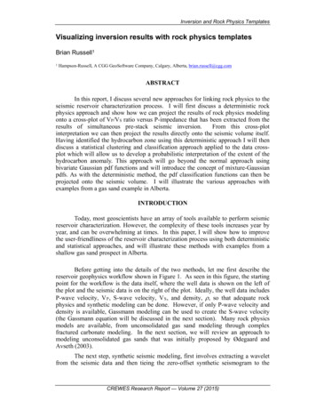
RussellFigure 19: Decision boundaries between the Vp/Vs ratio distributions of two different clusters for a North Africanwell example, where the ML decision boundary is shown on the left and the Bayesian decision boundary on theright.When we extend the clusters to two dimensions, we can write the bi-variateGaussian pdf as 1 1 T(14)exp ( x μk ) Σ k 1 ( x μk ) ,f(x, y ck ) 1/ 2 2 2π Σ k x where x is a vector containing the x and y measurements at a particular sample, y μkx μk is a vector containing the means of the x and y values in the kth cluster, μky σ kxx σ kxy and Σ k is the covariance matrix which contains the variances of the x σ kxy σ kyy and y data values in the kth cluster, σ kxx and σ kyy , on the main diagonal, and the1 Nk [(xi µkx )(yi µky )] , on the offN k 1 i 1diagonals. Equation 14 is the equation for an ellipse. Note that equation 14 can beextended to a multi-variate distribution of any dimension, which results in anellipsoid in three dimensions and a hyper-ellipsoid in more than three dimensions.Table 1 shows the bivariate statistics for the three cluster zones shown in Figure 11.covariance of the kth cluster, σ kxy Table 1: The statistics for the three clusters shown in Figure 11, which correspond to the red cluster on the left, theblue cluster in the middle and the green cluster on the right.CREWES Research Report — Volume 27 (2015)

Inversion and Rock Physics TemplatesUsing the statistics shown in Table 1, we then compute the bivariatedistributions given in equation 13, for each of the three clusters, and superimposethese elliptical surfaces on the points, as shown in Figure 20. Each ellipse representsthe points contained within a single standard deviation from the mean. Note that wehave gone out to two standard deviations but could have added more. Also note thatwe have superimposed the univariate distributions on top of the histograms shown inthe figure. On those distributions it is easy to see where the decision boundariesoccur.Figure 20: Bivariate elliptical Gaussian pdfs computed from the statistics in Table 1 and superimposed on theclusters of Figure 11, where each contour represents a single standard deviation.Next, we superimpose the bivariate Gaussian distributions shown in Figure 20back onto the seismic cross-section, as shown in Figure 21.Figure 21: The distributions shown in Figure 21 superimposed on the seismic cross-section.CREWES Research Report — Volume 27 (2015)

RussellThe colour scheme shown in Figure 21 can be interpreted as follows byreferring to both the bivariate and univariate distributions shown in Figure 20. Thestrongest colour represents the peak on the bivariate distribution, which occurs at themean value of each cluster. The colours are then scaled down to white based ondistance from the peak, until the decision boundary is reached. When the decisionboundary is reached, the colour on the scale changes to the next cluster colour.Next, we will extend our discussion to the mixture-Gaussian approach. In thisapproach, each cluster is modeled as the sum of J Gaussian pdf functions, given byJp(x, y ck ) w j f(x, y j) ,(15)j 1Jwhere the w j represent the weights on each individual pdf function, w j 1.0 andj 1 f ( x, y j )dxdy 1.0 .Table 2 shows the three Gaussian pdfs that went into ax, ymixture model for the first cluster in Figure 11. (We will not show the mixturemodels for the other two clusters since by showing one result we get the point across.)Note that the mixture weights are all very close to 1/3.Table 2: The statistics for the three Gaussian pdfs in the mixture model for cluster 1.The three pdfs shown in Table 2 are summed to produce the mixture-modelfor the first cluster, which is shown in Figure 22, as are the mixture models of theother two clusters. Again, note that the univariate distributions have beensuperimposed on top of the histograms shown in the figure. On those distributions itis clear that we now do not have a single Gaussian function, but instead have amixture of three. The choice of the number of pdfs to use in the mixture is controlledby the user. Obviously, as the number of pdfs increases, the fit to the cluster getstighter. However, including too many pdfs in the mixture can lead to “over-fitting”,in which noise or spurious points are fit too closely. Experience has shown that theuse of three pdfs in the mixture is a reasonable choice.CREWES Research Report — Volume 27 (2015)

Inversion and Rock Physics TemplatesFigure 22: Mixture-Gaussian pdfs superimposed on the clusters of Figure 11, where each contour represents asingle standard deviation.Finally, we project the mixture-Gaussian pdf functions shown inFigure 22 back onto the seismic cross-section, as we did in Figure 21 for the singlebivariate Gaussian pdf functions. This is shown in Figure 23. As in Figure 21, thecolour scheme shown in Figure 22 can be interpreted as follows by referring to boththe bivariate and univariate distributions shown in Figure 22. The strongest colourrepresents the peak on the bivariate distribution. However, unlike in the case of asingle bi-variate Gaussian, there are multiple peaks and valleys shown in the mixtureGaussian case. Thus, when the colours are then scaled down to white based ondistance from the highest peak on the distribution, there will be multiple regions ofthe distribution that get that colour, not just a level surface based on a single ellipss.As in Figure 20, when the decision boundary is reached, the colour on the scalechanges to the next cluster colour.Figure 23: The distributions shown in Figure 22 superimposed on the seismic cross-section.CREWES Research Report — Volume 27 (2015)

RussellNote that the statistical extent of the gas sand in Figure 23 is less than itsextent in Figure 22, which is probably related to the extra complexity added by themixture Gaussian approach. Which analysis you prefer (i.e. that of Figure 23 or 24)depends on which statistical fit you believe more.CONCLUSIONSIn this report, I discussed several new approaches allowing us to link a rockphysics template to pre-stack seismic inversion. In the first part of the talk I reviewedthe theory behind the deterministic rock physics template approach, specifically foran unconsolidated gas sand model. I then showed how we could project the

m sat sat K K K K K K K K K φ, (2 ) where K. sat. is the saturated bulk modulus, dry. is the dry bulk modulus, K. m. is the . K mineral bulk modulus and . φ is the porosity of the reservoir rock, and . f. is the bulk . K modulus of the reservoir fluid. To estimate the K. dry. value, we used the method proposed by Greenberg and .