Transcription
Hydrol. Earth Syst. Sci., 26, 2161–2180, 2022https://doi.org/10.5194/hess-26-2161-2022 Author(s) 2022. This work is distributed underthe Creative Commons Attribution 4.0 License.HESS Opinions: Chemical transport modelingin subsurface hydrological systems – space,time, and the “holy grail” of “upscaling”Brian BerkowitzDepartment of Earth and Planetary Sciences, Weizmann Institute of Science, Rehovot 7610001, IsraelCorrespondence: Brian Berkowitz (brian.berkowitz@weizmann.ac.il)Received: 27 October 2021 – Discussion started: 2 November 2021Revised: 16 March 2022 – Accepted: 30 March 2022 – Published: 28 April 2022Abstract. Extensive efforts over decades have focused onquantifying chemical transport in subsurface geological formations, from microfluidic laboratory cells to aquifer fieldscales. Outcomes of resulting models have remained largelyunsatisfactory, however, largely because domain heterogeneity – characterized for example by porosity, hydraulic conductivity and geochemical properties – is present over multiple length scales, and “unresolved”, practically unmeasurable heterogeneities and preferential pathways arise at virtually every scale. While spatial averaging approaches are effective when considering overall fluid flow, wherein pressurepropagation is essentially instantaneous, purely spatial averaging approaches are far less effective for chemical transport essentially because well-mixed conditions do not prevail. We assert here that an explicit accounting of temporal information, under uncertainty, is an additional but fundamental component in an effective modeling formulation.As an outcome, we further assert that “upscaling” of chemical transport equations – in the sense of attempting to develop and apply chemical transport equations at large lengthscales, based on measurements and model parameter valuesobtained at significantly smaller length scales – can be considered an unattainable “holy grail”. Rather, we maintain thatit is necessary to formulate, calibrate and apply models usingmeasurements at similar scales of interest.11.1IntroductionBackgroundThere have been extensive efforts over the last 60 years tomodel and otherwise quantify fluid flow and chemical (contaminant) transport in soils and subsurface geological formations, from millimeter-size, laboratory microfluidic cells toaquifer field scales extending to hundreds of meters and eventens of kilometers.Soils and subsurface formations typically exhibit significant heterogeneity in terms of domain characteristics such asporosity, hydraulic conductivity, structure, and biogeochemical properties (mineral and organic matter content). However, only more recently has it become broadly acceptedthat effects of heterogeneity over multiple length scales, with“unresolved”, practically unmeasurable heterogeneities arising at every length scale from pore to field, cannot simply be “averaged out”. Indeed, much research on flow andtransport in porous media, dating since 1950, has beenbased on the search for length scales at which one can definea “representative elementary volume” or otherwise-named“averaging volume”, above which variability in fluid andchemical properties becomes constant. In this context, too,many varieties of homogenization, volume averaging, effective medium, and stochastic continuum theories have beendeveloped in an extensive literature. These methods allowedformulation of continuum-scale, generally Eulerian, partialdifferential equations to quantify (“model”) fluid flow andchemical transport, which were then applied in the soil andgroundwater literature at length scales ranging from millimeters to full aquifers. While originally deterministic in char-Published by Copernicus Publications on behalf of the European Geosciences Union.
2162B. Berkowitz: HESS Opinions: Chemical transport modeling in subsurface hydrological systemsacter, a variety of stochastic formulations and Monte Carlonumerical simulation techniques, introduced from the 1980s,enabled analysis of uncertainties in input parameters such ashydraulic conductivity.However, while analysis of fluid flow using these methods has proven relatively effective, modeling of chemicaltransport, and an accounting of associated (biogeo)chemicalreactions in cases of reactive chemical species and/or hostporous media, has revealed serious limitations. We discussthe reasons for this in the sections below. Briefly, the overarching reason for these successes and failures is that spatialaveraging approaches are effective when considering overallfluid flow rates and quantities: pressure propagation is essentially instantaneous, and the system is “well mixed” becausemixing of water “parcels” is functionally irrelevant. However, purely spatial averaging approaches are far less effective for chemical transport, essentially because well-mixedconditions do not prevail, and spatial averaging is inadequate;here, an explicit, additional accounting of temporal effects isrequired.The focus of the current contribution is on modeling conservative chemical transport in geological media. In termsof modeling, one can delineate two main types of scenarios: (i) pore-scale modeling in relatively small domains, witha detailed and specified pore structure, and (ii) continuumscale modeling in porous media domains, which average porespace and solid phases at scales from laboratory flow cells tofield-scale plots and aquifers. Case (i) requires, e.g., Navier–Stokes or Stokes equation solutions for the underlying flowfield, coupled with solution of a local (e.g., advection–diffusion) equation for transport, while case (ii) requiresDarcy (or related) equation solutions for the underlying flowfield, coupled with solution of a governing transport equation for chemical transport. Note that, here and throughout,we shall use the terms continuum level and continuum scalein reference to case (ii) scenarios and pore scale to referto case (i) scenarios, although we recognize that pore-scaleNavier–Stokes and advection–diffusion equations, too, arecontinuum partial differential equations.Disclaimer: here and throughout this contribution, theoverview comments and references to existing philosophies,methodologies, and interpretations are written mostly inbroad terms, with only limited citations selected from thevast literature. This approach is taken with a clear recognition and respect for the extensive body of literature that hasdriven our field forward over the last decades but with theexpress desire to avoid any risk of unintentionally alienatingcolleagues and/or misrepresenting aspects of relevant studies. As an Opinions contribution, and with length considerations in mind, there is no attempt to provide an exhaustivelisting and description of the relevant literature.Hydrol. Earth Syst. Sci., 26, 2161–2180, 20221.2AssertionsThe pioneering paper of Gelhar and Axness (1983) focusedon quantifying conservative chemical transport at the continuum level. They expressed heterogeneity-induced chemicalspreading in terms of the (longitudinal) macrodispersion coefficient – as it appears in the classical (macroscopically 1D)advection–dispersion equation – with knowledge of the variance and correlation length of the log-hydraulic conductivity field and the mean, ensemble-averaged fluid velocity. Theconceptual approach embodied in Gelhar and Axness (1983)– and by many researchers since then (as well as previously)– was founded on delineation of the spatial distribution ofthe hydraulic conductivity and application of an averagingmethod to yield a governing transport equation with “effective parameters” that describes chemical transport at a givenlength scale (e.g., Dagan, 1989; Gelhar, 1993; Dagan andNeuman, 1997).In contrast, we assert here that spatial information, alone,is generally insufficient for quantification of chemical transport phenomena. Rather, temporal information is an additional, but fundamental, component in an effective modeling formulation. In the discussion below, we shall justify thisargument by a series of examples. We examine (i) spatial information on, e.g., the hydraulic conductivity distribution atthe continuum level or distribution of the solid phase at thepore-scale level and (ii) temporal information on, e.g., contaminant (tracer, “particle”) transport mobility and retentionin different regions of a domain. We thus define a type of“information hierarchy”, with different types of informationrequired for different flow and chemical transport problemsof interest.As an outcome of the above assertion and the discussionbelow, we further assert that “upscaling” of chemical transport equations – development and application of chemicaltransport equations at large (length) scales, with corresponding parameter values, based on measurements and model parameter values obtained at significantly smaller length scales– can be considered an unattainable “holy grail”. Rather, wemaintain that it is necessary to formulate and calibrate models and then apply them over spatial scales with relativelysimilar orders of magnitude. This does not exclude use ofsimilar equation formulations at different spatial scales, butit does entail use of different parameter values, at the relevantscale of interest, that cannot be determined a priori or frompurely spatial or flow-only measurements.1.3Approach – outlineWhile our focus is on chemical transport, knowledge of fluidflow and delineation of the velocity field throughout the domain is a prerequisite. We therefore first discuss fluid flow asan intrinsic element of the “information hierarchy”. Specifically, we address the 2
B. Berkowitz: HESS Opinions: Chemical transport modeling in subsurface hydrological systems1. How basic structural information on “conducting elements” in a system representing a porous and/or fractured geological domain can provide insight regardingoverall fluid conduction in the domain as a function ofconducting element density. We emphasize that withoutdirect simulation of fluid flow in such a system, this typeof analysis does not delineate the actual flow field andvelocity distributions throughout the domain.2. How spatial information on the hydraulic conductivitydistribution at a continuum scale, or solid-phase distribution at the pore scale, throughout the domain, can beused to determine the flow field. We then show that thisis insufficient to define chemical transport.3. How temporal information on chemical species migration, which quantifies distributions of retention andrelease times (or rates) of chemicals by advective–dispersive–diffusive and/or chemical mechanisms, canbe used to determine the full spatial and temporal evolution of a migrating chemical plume, either by solutionof a transport equation or use of particle tracking on thevelocity field.We comment, parenthetically, that in conceptual–philosophical terms, this hierarchy and the limitationsof each level are in a sense analogous to representation ofgeometrical constructs in multiple dimensions: in principle,one can represent, as a projection, a d-dimensional object ind 1 dimensions. However, of course, by its very nature, aprojection does not capture all features of the construct in its“full” dimension. To illustrate this, an imaginary 1D curvecan represent a 2D Möbius strip, a 2D perspective drawingcan represent a 3D cube, and a 3D construct can represent a4D object (where the fourth dimension might be time), andyet none of these d 1-dimensional representations containsall features of the actual d-dimensional objects. Similarly,despite our frequent attempts to the contrary, one cannotproperly describe (2) only from (1) or (3) only from (2).2Fluid flowAnalysis of the geometry of structural elements in a domaincan yield basic insights into fluid flow patterns. This approach is used, for example, when examining fracture networks in essentially impermeable host rock. As discussedbelow, however, full delineation of the underlying velocityfield ultimately requires solution of equations for fluid flow.In this context, percolation theory (Stauffer and Aharony,1994) is particularly useful in determining, statistically,whether or not a domain with N conducting elements (e.g.,fractures) includes sufficient element density to form a connected pathway enabling fluid flow across the domain. Onecan estimate, for example, (i) the critical value, Nc , for whichthe domain is “just” connected, as a function of 163length distribution or (ii) the critical average fracture lengthas a function of N needed to reach domain connectivity(Berkowitz, 1995). Similarly, percolation theory shows howthe overall hydraulic conductivity of the domain scales as thenumber of conducting elements, N , relative to the Nc critical number of conducting elements required for the systemto begin to conduct fluid. Percolation theory also addressesdiffusivity scaling behavior of chemical species. However,fundamentally, percolation is a statistical framework suitable for large (“infinite”) domains and provides universalscaling behaviors with no coefficient of equality; see, e.g.,Sahimi (2021) for detailed discussion.Other approaches have been advanced to analyze domain connectivity, for example, using graph theory and concepts of identification of paths of least resistance in porousmedium domains (e.g., Rizzo and de Barros, 2017) or topological methods (e.g., Sanderson and Nixon, 2015). Like percolation theory, such approaches provide useful informationon and “estimates” of the hydraulic connectivity and flowfield, and even of the first arrival times of chemical species,without solving equations for fluid flow and chemical transport. However, these methods do not provide full delineationof the flow field and velocity distribution throughout a domain.These considerations indicate that, in general, dynamic aspects of fluid flow are critical: knowledge of pure geometryis not sufficient, and we must actually solve for the flow field,at either the pore scale or continuum scale, to determine thevelocity field and actual flow paths throughout the domain.Delineation of a flow field and velocity distribution by solution of the Navier–Stokes equations (or Stokes equation forsmall Reynolds numbers) or by solution of the Darcy equation may be considered rigorous, correct, and effective. However, in the process of solving for the flow field, two key features arise, one more relevant to pore-scale analyses and theother more relevant to continuum-scale analysis, as detailedin Sect. 2.1 and 2.2, respectively.2.1Pore-scale flow field analysisWhy is knowledge only of the geometrical “static” structure(spatial distribution of the solid phase) insufficient to knowthe flow dynamics in a pore-scale domain? Consider the 2Ddomain shown in Fig. 1, containing sparsely and randomlydistributed obstacles (porosity of 0.9). Figure 1 shows solutions of the Navier–Stokes equations for two Reynolds number (Re) values. Recall that Re ρvL/µ, where ρ and µ aredensity and dynamic viscosity of the fluid, respectively, v isfluid velocity, and L is a characteristic linear dimension. Hereand throughout, the fluid is assumed to have constant viscosity. Andrade et al. (1999) showed clearly that well-definedpreferential flow channels at lower Re, while at higher Re,channeling is less intense and the streamline distribution ismore spatially homogeneous in the direction orthogonal tothe main flow. The domain shown in Fig. 1 is not intendedHydrol. Earth Syst. Sci., 26, 2161–2180, 2022
2164B. Berkowitz: HESS Opinions: Chemical transport modeling in subsurface hydrological systemsto represent a natural geological domain but rather to illustrate streamline behavior in even relatively simple pore-scalegeometries.Figure 1 demonstrates that the streamlines in individualpores change because of the interplay between inertial andviscous forces given by Re. In other words, with a changein overall fluid velocity or hydraulic gradient across the domain, the actual flow paths can be altered, together with achange in overall and (spatially) local residence times of fluidmolecules; the same factors also govern chemical species, asaddressed below. Of course, the significantly lower porositiesand more tortuous pore space configuration in natural, heterogeneous geological porous media may affect the impactof inertial effects, especially at the pore scale, but the principle remains relevant. We note, too, parenthetically, that thebehavior shown in Fig. 1 is also relevant to fluid flow withinfracture planes, wherein the obstacles represent contact areasand regions of variable aperture.Clearly, then, except in highly idealized and simplified geometries, use of a purely analytical solution to identify thefull velocity field and streamline patterns at the pore scale isnot feasible. Moreover, the extent and changes in streamlinesare not intuitively obvious without full numerical solution ofthe governing flow equations, for any specific set of porousmedium structures and boundary conditions.2.2Continuum-scale flow field analysisConsidering now continuum-scale domains, but in analogyto the example shown in Sect. 2.1, we illustrate why knowledge only of the geometrical “static” structure is insufficientto know the flow dynamics, without solution of the Darcyequation. Here, the geometrical structure refers to the spatialdistribution of the hydraulic conductivity, K.Figure 2 represents a realization of a numerically generated (statistically homogeneous, isotropic, Gaussian) hydraulic conductivity 2D domain. The Darcy equation solution for this domain yields values of hydraulic head throughout the domain; these are converted to local velocities toenable delineation of the streamlines and preferential flowpaths. The latter are highlighted by actually solving forchemical transport by following the migration of “particles”representative of masses of dissolved chemical species injected along the inlet boundary of the flow domain; see Edery et al. (2014) for details. Of particular significance is that99.9 % of the injected particles travel in preferential pathways through a limited number of domain cells. We returnto Fig. 2 in Sect. 3.3.2, where we discuss a framework thateffectively characterizes and quantifies chemical transport.Unlike the pore-scale case shown in Sect. 2.1, at the Darcy/continuum scale, streamlines are not altered with changesin the overall hydraulic gradient as long as laminar flow conditions are maintained. And yet, preferential flow paths are(possibly surprisingly) sparse and ramified, sampling onlylimited regions of a given heterogeneous domain, with theHydrol. Earth Syst. Sci., 26, 2161–2180, 2022vast fraction of a migrating chemical species that interrogatesthe domain being even more limited. Significantly, exceptin highly idealized and simplified geometries, delineation ofthese pathways is not intuitively obvious (e.g., by simple inspection of the hydraulic conductivity map in Fig. 2a) or definable from a priori analysis or tractable analytical solution.Rather, numerical solution of the governing flow equationsis required for any particular/specific set of porous-mediumstructures and boundary conditions. Note, too, that criticalpath analysis from percolation theory (discussed in Sect. 2)– again from purely “static” information without solution ofthe flow field – yields an incorrect interpretation, as shown indetail by Edery et al. (2014).We emphasize that the delineation of “preferential flowpaths” is usually relevant only for study of chemical transport; if water quantity, alone, is the focus, then specific “flowpaths” traveled by water molecules – and their advective anddiffusive migration along and between streamlines and into/out of less mobile regions – are of little practical interest.On the other hand, the movement of chemical species, whichexperience similar advective and diffusive transfers, must bemonitored closely to be able to quantify overall migrationthrough a domain. We return to considering patterns of chemical migration in Sect. 3. This argument, too, reinforces theassertion that delineation of actual chemical transport cannot be deduced purely from spatial information and solutionfor fluid flow but must be treated by solution of a transportequation.It is significant, too, that fluid flow and chemical transportoccur in preferential pathways that contain low-conductivitysections (indicated by circles in Fig. 2c and d). How do weexplain passage through low-hydraulic-conductivity “bottlenecks” within the preferential pathways rather than migration“only” through the highest-conductivity patches?To address this question, we first consider what happensin a 1D path. Consider two paths, each containing a seriesof five porous-medium elements or blocks, with distinct hydraulic conductivity values, Ki . Consider Path 1, with a series of hydraulic conductivity values of 3, 3, 3, 3, and 3,and Path 2, with values 6, 6, 1, 6, and 6 (specific length/time units are irrelevant here). The value of K 1 represents a clear “bottleneck” in an otherwise higher-K paththan that of Path 1. In a 1D series, however, the overall hydraulic conductivity (Koverall ) of the path is given by the harmonic mean of the conductivities of the elements comprisingthe path: Koverall 5/(6i 1,5 1/Ki ). Significantly, in the twocases here, both paths have Koverall 3. So, a “bottleneck”(K 1) can be “overcome” and does not cause necessarily apotential pathway to be less “desirable” than a pathway without such “bottlenecks”. In other words, flow through pathways containing some low-K regions should be expected.Of course, in 2D and 3D systems, patterns of heterogeneity and pathway “selection” by water/chemicals are significantly more complicated, but the principle discussed herefor 1D systems still holds in the sense that 1-2022
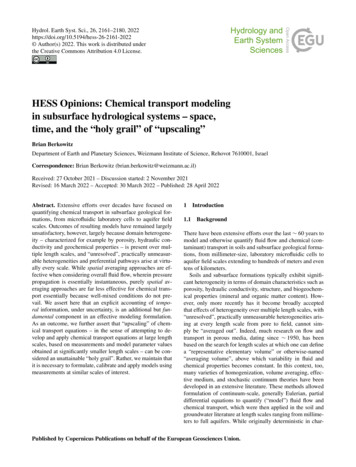
B. Berkowitz: HESS Opinions: Chemical transport modeling in subsurface hydrological systems2165Figure 1. Two-dimensional domain containing randomly distributed obstacles (squares and rectangles). Stream functions for (a) Re 0.0156and (b) Re 15.6 are shown with constant increments between consecutive streamlines (from Andrade et al., 1999; copyright AmericanPhysical Society). The different patterns of preferential pathways are clear and distinct. The three pairs of circles (red, blue, black) highlightthree (of many) specific locations where the streamlines are seen to change as a function of Re.conductivity (“bottleneck”) elements can (and do) exist in thepreferential pathways (e.g., Margolin et al., 1998; Bianchi etal., 2011).3Chemical transportWe now consider the next level of the “information hierarchy” outlined in Sect. 1.3. To quantify the evolution of a migrating chemical plume, knowledge of the flow field is notgenerally sufficient, and additional means to characterize andquantify the behavior are needed. Dynamic aspects of chemical transport require us to think (also) in terms of time, notjust space and physical structure. Moreover, it is generallyinsufficient to determine the transport of the chemical plumecenter of mass. Rather, in terms of water resource contamination and remediation, for example, it is critical to characterize, respectively, the early and late arrival times in compliance or monitoring regions downstream of the point, areal,or volumetric regions in which the chemical species enteredthe system.As we show below, it becomes clear that there are dynamicaspects of chemical transport, over and above the role of theflow field: we must actually solve for chemical transport, ateither the pore scale or continuum scale, to determine thespatial plume and/or temporal breakthrough curve evolutionof the migrating chemical plume. In both the pore-scale andcontinuum-scale domains, the critical control that arises isthat of time, in addition to space. This is in sharp contrastto fluid flow at the pore and continuum scales, as shownin Sect. 2.1 and 2.2: pore-scale fluid flow displays changing streamlines with changes in hydraulic gradient, whilecontinuum-scale fluid flow follows distinct but difficult-toidentify preferential flow paths essentially independent of thehydraulic We point out, too, that for both pore-scale and continuumlevel scenarios, one can solve explicitly a governing equation for transport. Alternatively, one can obtain an “equivalent” solution by solving for “particle tracking” of transportalong the calculated streamlines, in a Lagrangian framework.In other words, particle tracking methods essentially represent an alternative means of solving an (integro-)partial differential equation for chemical transport; such methods canbe applied, too, when the precise partial differential equationis unknown or the subject of debate. We also note that solution of the relevant equations for fluid flow and chemicaltransport is sometimes achieved by (semi-)analytical methods if the flow/transport system can be treated sufficientlysimply (e.g., as macroscopically, section-averaged 1D flowand transport in a rectangular domain).We first discuss principal features of pore-scale (Sect. 3.1)and continuum-scale (Sect. 3.2) chemical transport, and inSect. 3.3, we focus on effective model formulations. We focus on conservative chemical species and mention chemical reaction effects only peripherally. Note that other factors such as temporally/spatially changing fluid viscosity andsurface tension, or mechanical and wetting properties of thesolid phase, represent further complexities that are not considered here.3.1Pore-scale chemical transport analysisTo illustrate why knowledge only of the flow field is insufficient for full quantification of chemical transport, consider the three porous-medium domains shown in Fig. 3.Each domain is comprised of pore-scale images of a naturalrock, modified by enlarging the solid-phase grains, to yieldthree different configurations: a statistically homogeneoussystem domain, a weakly correlated system, and a structured,strongly correlated system (see Nissan and Berkowitz, 2019,for details). Fluid flow was determined by solution of theHydrol. Earth Syst. Sci., 26, 2161–2180, 2022
2166B. Berkowitz: HESS Opinions: Chemical transport modeling in subsurface hydrological systemsFigure 2. Maps of (a) hydraulic conductivity, K, distribution in a domain with 300 120 cells, (b) preferential pathways for fluid flow (andchemical transport), and (c) preferential pathways through cells that each contain a visitation of at least 0.1 % of the total number of chemicalspecies particles injected into the domain (flux-weighted, along the entire inlet boundary). Flow is from left to right. Note that the colorbars are in ln(K) scale for (a) and log10 number of particles for (b, c) (Edery et al., 2014; with permission from the American Geophysical Union 2014). (d) Laboratory flow cell (dimensions 2.13 (length) 0.65 (height) 0.10 (width) m) with an exponentially correlated Kstructure, showing preferential pathways for blue dye injected near the inlet (flow is left to right); dark-, medium-, and light-colored sandsrepresent high, medium, and low conductivity, respectively (Levy and Berkowitz, 2003; with permission from Elsevier 2003). The circlesshown in (c) and (d) highlight two (of many) regions in which the pathways are seen to contain lower K “bottlenecks”.Navier–Stokes equations (Fig. 1a). Transport of a conservative chemical species was then simulated via a (Lagrangian)streamline particle tracking method for an ensemble of particles that advance according to a Langevin equation. Transport behavior was determined for two values of the macroscopic (domain-average) Péclet number (P e). Recall thatP e vL/D, where v is fluid velocity, L is a characteristiclinear dimension, and D is the coefficient of molecular diffusion. Here, the macroscopic P e is based on the mean particlevelocity and mean particle displacement distance per transition (or “step”).Hydrol. Earth Syst. Sci., 26, 2161–2180, 2022Figure 3 shows that, regardless of possible pore-scalestreamline changes as a function of hydraulic gradient (recallSect. 2.1, considering different values of Re), the choice ofmacroscopic Péclet number in a given domain plays a significant role in the evolution of the migrating chemical plume.In particular, the relative effects of advection and diffusion,which vary locally in space, are critical, as is the overall residence time in the domain. We stress here, and return to thiskey point in the discussion below, that the spatially and insome cases temporally local changes in relative effects ofadvection and diffusion – characterized by the local P e –https://doi.org/10.5194/hess-26-2161-2022
B. Berkowitz: HESS Opinions: Chemical transport modeling in subsurface hydrological systems2167Figure 3. Fluid velocities and chemical migration in three porous media configurations (from left to right): homogeneous system, randomlyheterogeneous system, and structured heterogeneous system. The upper row shows the (normalized) velocity field for the three configurations; the color bar represents relative velocity, with dark blue being lowest. The middle and lower rows show, respectively, numericallysimulated particle tracking patterns of an inert chemical species (blue dots) at P e 1 (middle row) and P e 100 (lower row) for thethree configurations (white color indicates solid phase; black color indicates liquid phase). Each system has overall dimensions of 8 cm(length) 6 cm (height). Note: the particle plumes are shown at 10 % of the final time of each simulation; absolute travel times differ amongthe plots. The insets in the left-hand-side plots of the middle and lower rows show the pore-scale chemical species distributions; note themore diffuse pattern for P e 1 (from Ni
numerical simulation techniques, introduced from the 1980s, . pore-scale modeling in relatively small domains, with a detailed and specified pore structure, and (ii) continuum-scale modeling in porous media domains, which average pore space and solid phases at scales from laboratory flow cells to field-scale plots and aquifers. Case (i .